Marketing Mix Modeling Forecasting Needs More Than Historical Fit

Marketing mix modeling forecasting fails when teams treat historical model fit as proof of future performance. Marketing mix modeling (MMM) is a statistical method that uses historical aggregate data to measure media impact. A model can fit past revenue numbers with high precision. That same model can make dangerous mistakes during budget planning. To generate a reliable marketing revenue forecast, teams must separate three tasks: historical prediction, causal contribution, and scenario forecasting.

A high goodness-of-fit score shows only that a statistical formula can reproduce known past results. It does not prove that the model identified true cause and effect. If you shift your marketing investments based on correlation rather than true lift, your media mix forecast will degrade. Lift is the incremental change in sales that paid advertising causes. Reliable marketing spend forecasting requires explicit baseline controls, disciplined response boundaries, uncertainty intervals, and continuous backtesting.

Three Forecasting Jobs

Marketing measurement uses different tools to answer different questions. Confusion between these tools creates planning errors. Teams frequently mix three distinct methods:

1. Digital attribution tracks observed user touchpoints through digital identifiers. Attribution assigns credit for a sale to specific marketing ads along a customer journey. It helps operators evaluate short-term campaign paths, but it struggles with signal loss, view-through claims, and cross-device tracking.
2. Incrementality testing creates controlled experiments, such as randomized geographic holdouts. It provides causal proof over a specific test window.
3. Marketing mix modeling uses aggregate historical time-series data to evaluate baseline trends, channel contributions, and saturation curves.

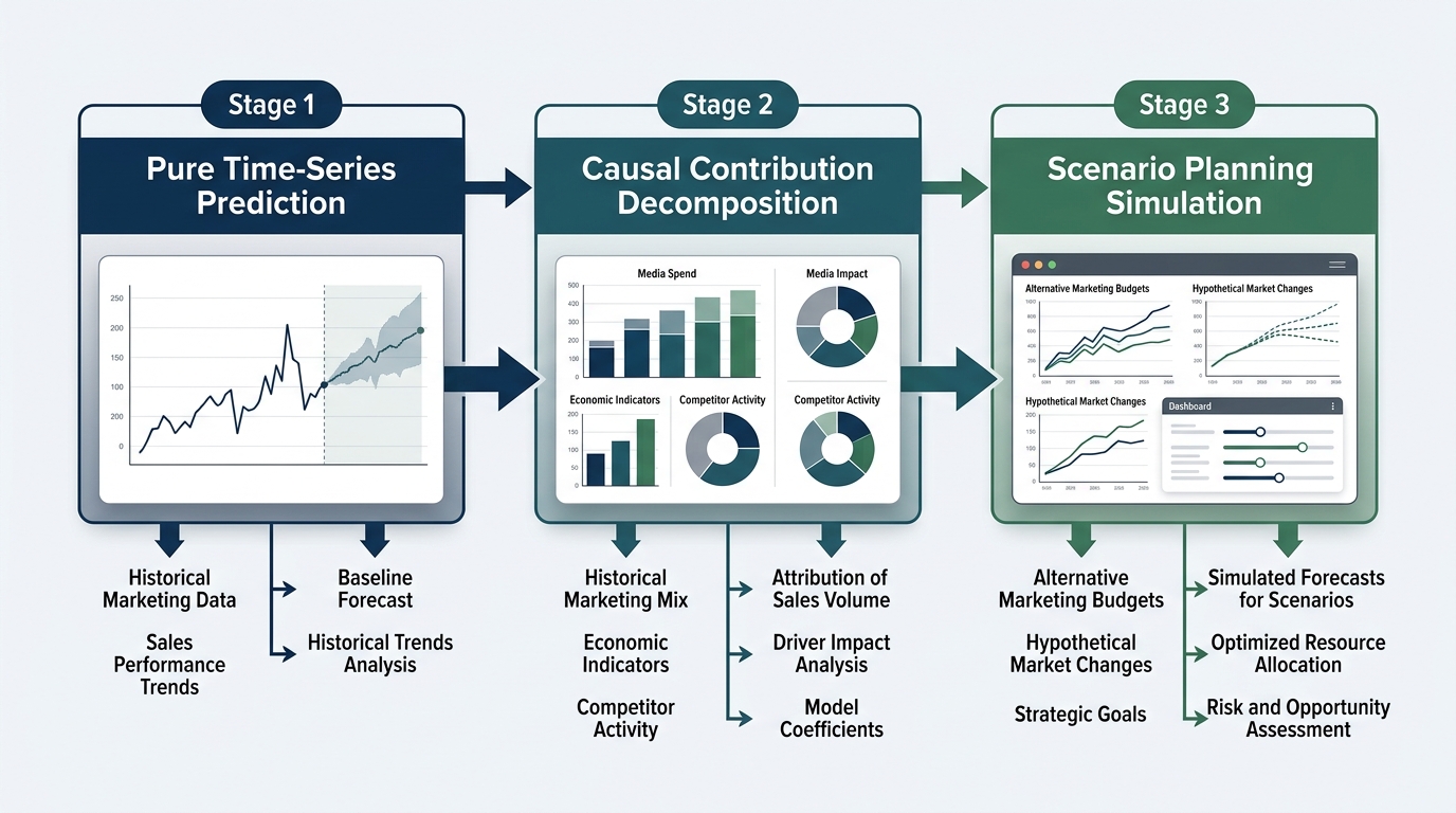
When you use marketing mix modeling for planning, you must recognize three separate forecasting jobs:

First, pure time-series prediction asks: what will total sales be if all current conditions continue without change? A standard time-series model can answer this question without marketing data.

Second, causal contribution estimation asks: how much past revenue did each marketing dollar create? The econometric specification estimates parameters for adstock and saturation. Adstock measures the carryover duration of advertising impact. Saturation reflects diminishing marginal returns, where each added dollar produces less revenue. The measurement team at getrecast.com explains that an MMM must model why sales occur. Simple predictive models capture correlations that collapse when you alter spend.

Third, scenario planning asks: what will happen if we spend different amounts across specific channels next quarter? This is the primary business purpose of an MMM forecast. It requires you to simulate future actions under untested external conditions. Good historical prediction does not guarantee good scenario predictions.

Forecasting Job	Primary Question	Core Risk	Primary Metric
Pure Time-Series Prediction	What will sales be if past patterns continue?	Ignores marketing mix changes	Holdout MAPE / RMSE
Causal Contribution	Which historical dollars drove incremental sales?	Confounding and spurious correlation	Experimental lift test alignment
Scenario Planning	What revenue will a new budget allocation generate?	Out-of-sample extrapolation failure	Continuous interval coverage

Baseline Forecast

An MMM separates revenue into two broad categories: incremental marketing contribution and baseline demand. Baseline demand represents sales that occur without paid marketing support. It includes brand equity, organic traffic, seasonality, economic trends, and promotional pricing.

A safe marketing revenue forecast starts with a realistic baseline. If your baseline estimate is incorrect, your media contribution estimates will also be incorrect. For example, if your baseline ignores macroeconomic inflation or competitive price cuts, the model will attribute those demand changes to your media channels.

You cannot run a future media mix forecast without future values for your control variables. An MMM estimates how controls influence sales, but it does not project those controls forward on its own. As documented by researchers at subconscious.ai regarding control forecasting pipelines, teams must forecast external controls through dedicated models before simulating media scenarios.

Open-source implementations show how to execute this process correctly. The engineering team at pymc-marketing.io demonstrates coupling foundation forecasting models with MMM architectures to project external covariates into future quarters.

When you configure your baseline, use this sequence:

1. Identify exogenous controls that drive organic demand, including holidays, seasonality indices, competitor prices, and macroeconomic indicators.
2. Build dedicated time-series projections for each exogenous control over the planning horizon.
3. Validate that your baseline demand aligns with organic brand sales during periods when major paid media channels were dark.
4. Review the relationship between your baseline specification and your media budget optimization guide to avoid overstating the revenue that paid spend can generate.

Media Scenarios

Once the baseline demand is stable, teams can model future media spend. A media mix forecast applies mathematical transformation functions to planned channel spend. These functions capture two real-world marketing dynamics: carryover effects and diminishing returns.

The model calculates carryover effects through adstock decay. The equation below shows a standard geometric decay transformation:

$$A_t = x_t + \lambda A_{t-1}$$

In this formula, $x_t$ represents the marketing spend at time $t$, and $\lambda$ represents the decay parameter between zero and one. This formula calculates how much advertising exposure from prior weeks influences consumer behavior today.

Next, the model calculates saturation through a nonlinear diminishing returns curve, such as the Hill function:

$$S(A_t) = \frac{A_t^\gamma}{K^\gamma + A_t^\gamma}$$

Here, $K$ represents the half-saturation point, and $\gamma$ controls the shape of the curve. As channel spend increases, each additional dollar generates less incremental sales volume. A thorough evaluation of these curves appears in the marketing response curves documentation.

A budget scenario forecast combines these transformations across all active channels. Consider this hypothetical quarterly budget plan:

• Channel A (Search): Spend increases from $100,000 per month to $150,000 per month. The model shows high current efficiency, but the spend approaches the steep inflection point of the Hill curve.
• Channel B (Paid Social): Spend stays flat at $200,000 per month. The model shows stable returns with low decay.
• Channel C (Video): Spend decreases from $80,000 to $30,000 per month. The model indicates long decay. Past video impressions will support demand for several weeks after the reduction.

When you run these inputs through the fitted model parameters, the engine sums the baseline sales and the incremental media sales. This produces the projected marketing revenue forecast.

Out-of-Range Risk

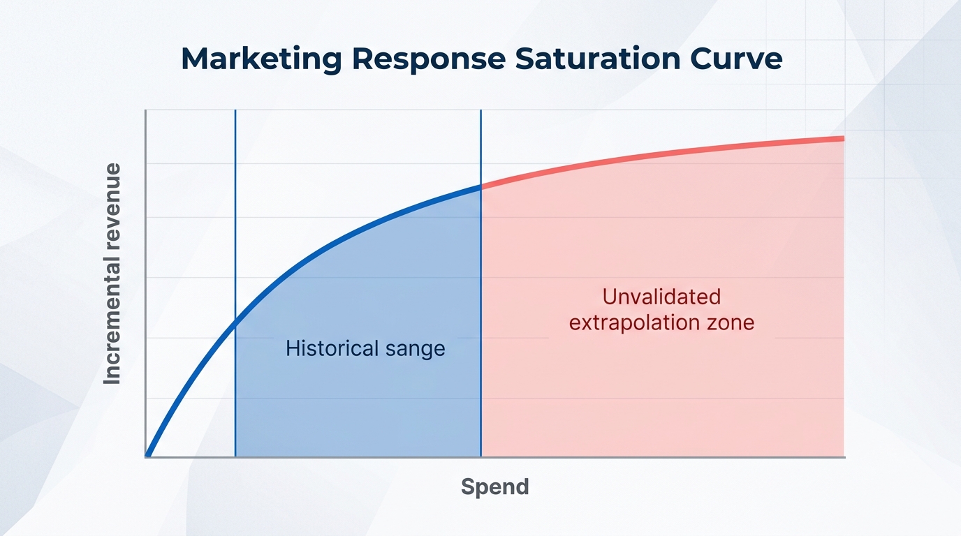
A marketing mix model is an empirical interpolation system. It learns patterns from historical variation. When business leaders propose drastic budget changes, they push the model into dangerous territory.

The measurement methodology review from ekimetrics.com describes how regression engines decompose historical revenue drivers, but regression engines cannot confirm outcomes outside historical observations. If a channel historically operated between $20,000 and $40,000 per week, the model has no empirical data for a $120,000 weekly budget.

Extrapolation risk manifests in three distinct ways:

• Saturation Curve Collapse: The mathematical curve forces a trajectory based on the chosen prior distribution rather than real consumer behavior. The model may predict massive incremental revenue, or it may force false saturation early.
• Auction Dynamics Shift: Drastic spend increases change your marginal cost per thousand impressions (CPM). An MMM calibrated on low-spend auctions cannot predict clearing prices in high-spend auctions.
• Channel Interaction Distortions: Massive changes in one channel alter the performance of other channels. A large reduction in upper-funnel video spend eventually erodes the conversion efficiency of branded search.

To avoid dangerous planning assumptions, enforce operational boundaries on all scenarios. Cap simulated channel shifts within 20% to 30% of their historical spend range. When a business scenario requires spending beyond those historical limits, run an incrementality field experiment first. Use the lift test results to recalibrate the response curves before you finalize the forecast.

Intervals and Sensitivity

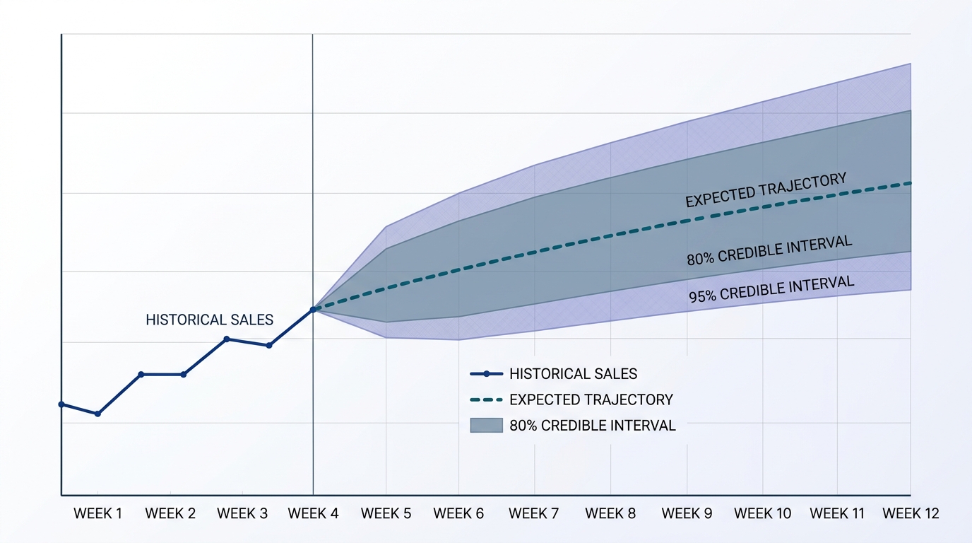
Deterministic forecasts provide a single number, such as: "A $2,000,000 marketing budget will generate $8,450,000 in revenue." Single-point forecasts create a false sense of certainty. Modern measurement requires a probabilistic approach.

Bayesian marketing mix models produce posterior distributions for every parameter. Instead of a single return value, the model provides credible intervals. A proper scenario forecast presents expected outcomes alongside 80% or 95% uncertainty intervals. As noted by analytics practitioners at thestacc.com in their measurement planning guide, reporting wide intervals prevents overconfidence. It prompts teams to run field tests before committing large capital outlays.

Forecast uncertainty stems from three main components:

1. Parameter Uncertainty: The model does not know the exact saturation threshold or adstock rate. The Bayesian posterior captures this range of possible values.
2. Control Covariate Uncertainty: The baseline projections for competitor actions, weather, or economic conditions carry their own statistical errors.
3. Residual Variance: Random variation and unmeasured market noise remain in the system.

A scenario analysis must also include sensitivity testing. A sensitivity test alters key assumptions systematically to observe the impact on revenue outcomes. Return on ad spend (ROAS) measures gross revenue generated for each dollar of ad spend.

Scenario Condition	Planned Spend Shift	Assumed Baseline Trend	Projected ROAS (80% Interval)	Strategic Action
Optimistic	+15% across top channels	+5% economic growth	2.4x (2.1x – 2.7x)	Scale budget with weekly pause triggers
Expected	Base plan allocation	0% macroeconomic drift	1.9x (1.6x – 2.2x)	Execute current operational plan
Conservative	-10% reallocation to search	-3% economic headwind	1.5x (1.1x – 1.8x)	Protect baseline cash flow

Communicate these intervals directly to finance leaders. When leadership understands the full spread of potential outcomes, they can build realistic contingency plans.

Backtesting

Never deploy a media mix forecast without proving its out-of-sample predictive validity. Many models look exceptional on paper because they overfit past data. A model with an $R^2$ of 0.95 can fail completely when predicting future quarters.

Standard cross-validation methods that randomly hold out single days or weeks are invalid for marketing mix modeling. Randomly holding out individual rows turns time-series prediction into an interpolation task. The model uses surrounding days to guess the missing date, which hides true model drift.

Proper validation requires contiguous holdout periods. In their technical guide on model validation, getrecast.com details how contiguous time-series holdout checks expose model failure. The checks require the engine to predict forward blocks of time that it has never seen.

Follow this backtesting protocol:

1. Select a historical cutoff date, such as twelve weeks before your latest data point.
2. Train the model using only the information available before that cutoff date.
3. Supply the planned spend and actual controls for the next twelve-week block.
4. Generate the forward projection and compare the predicted distribution against actual sales.
5. Review the guidelines to validate your MMM across multiple rolling windows to verify stability across seasons.

Score your backtests using point metrics and distributional metrics. Calculate Mean Absolute Percentage Error (MAPE) to monitor central accuracy. Concurrently, measure interval calibration. Across many rolling backtests, an 80% credible interval should contain the actual realized sales about 80% of the time. If actual sales fall inside your interval only 30% of the time, your model is overconfident. If actual sales fall inside the interval 99% of the time, your model bands are too wide to guide decisions.

Bounded Planning Scenarios

Marketing mix modeling forecasting provides valuable strategic guidance when teams respect its mathematical limits. Historical fit measures how well a formula describes the past. It does not prove causal attribution, and it does not protect against extrapolation errors.

To plan your upcoming media investments safely, build bounded planning scenarios. Do not rely on single unconstrained optimizations. Define explicit minimum and maximum boundaries for each channel based on historical exposure. State your baseline economic assumptions directly, present full credible intervals to executive stakeholders, and recalibrate your response curves through continuous geographic holdout tests.