A Marketing Response Curve Is Not a Forecast

A marketing response curve shows how incremental sales change when you increase channel spend. Incremental sales are the additional sales that marketing causes. The curve does not predict future revenue with certainty. Instead, this mathematical function maps past spend to expected incremental returns under fixed market conditions.

Teams often confuse response curves with forecasts. A forecast projects total revenue forward across calendar time, seasonal shifts, competitor moves, and operational limits. A media response curve isolates how one marketing channel behaves at different spend levels. It assumes that other variables do not change. When media planners treat a marketing response curve as an unconditional forecast, they overspend on saturated channels. They also set unrealistic sales goals.

       Response Curve vs. Media Forecast
┌────────────────────────┬────────────────────────┐
│ Response Curve (MMM)   │ Media Forecast         │
├────────────────────────┼────────────────────────┤
│ Static snapshot        │ Time-series projection │
│ Isolates one channel   │ Mixes all growth drivers│
│ Assumes ceteris paribus│ Models changing context│
│ Sets marginal targets  │ Sets revenue targets   │
└────────────────────────┴────────────────────────┘

presenc.ai defines a marketing response curve as the function that maps channel spend to incremental business outcomes. It calculates outcomes after it applies adstock and saturation transformations. It provides the foundation for budget optimization, not a timeline of actual weekly sales.

Response Curve Anatomy

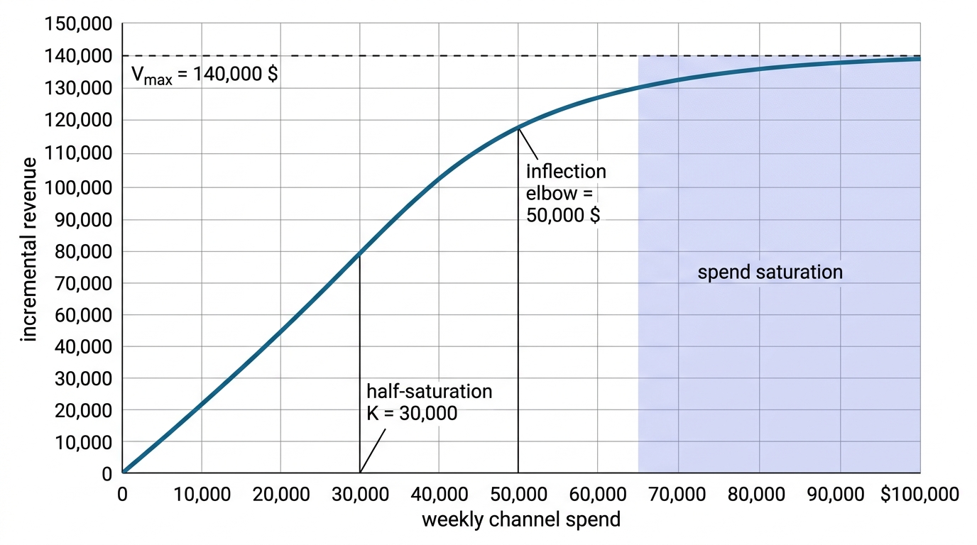
An advertising saturation curve usually follows an S-shape or a concave curve. Saturation occurs when additional ad spend produces smaller gains. In modern marketing mix models, data scientists frequently select the Hill function to represent diminishing returns in advertising. Marketing mix modeling uses statistical analysis on aggregate past data to estimate marketing effects.

The standard Hill function uses three core parameters:

$$\text{Response}(x) = V_{\max} \cdot \frac{x^n}{K^n + x^n}$$

In this formula:

• $x$ represents media input, such as spend or adstocked impressions.
• $V_{\max}$ represents the asymptote, or the maximum possible incremental response from this channel.
• $K$ represents the half-saturation point. This point is the spend level that produces 50 percent of $V_{\max}$.
• $n$ represents the shape parameter. When $n > 1$, the function creates an S-curve with initial increasing returns. When $n \le 1$, the curve remains concave.

Brian Curry explains in his digital media optimization analysis that these three parameters control the upper ceiling, scale, and steepness of media response.

The shape of the channel response function changes as spend increases:

1. Initial Region: At very low spend, the curve can be flat if an S-curve applies. It is steep if a concave curve applies. Small budgets often fail to create measurable consumer awareness.
2. Linear Growth Region: Spend increases create proportional sales gains. The slope here represents high marginal efficiency.
3. Elbow or Diminishing Return Region: Each new dollar generates less incremental sales than the prior dollar. The slope begins to flatten.
4. Saturation Asymptote: The channel reaches complete spend saturation. Additional spend generates almost zero new incremental revenue. The audience has reached total exposure frequency.

Adstock Before Saturation

You must apply transformations in the correct sequence when you build marketing mix model response curves. Models must always calculate the adstock transformation before they calculate saturation.

Adstock reflects consumer memory and sales carryover over time. Saturation reflects audience exhaustion within a specific period. Media delivery creates ad impressions that persist in consumer memory across multiple weeks. Diminishing returns occur when consumers experience high cumulative exposure.

Metricgate outlines the mathematical necessity of applying adstock first because carryover operates on raw media delivery. In contrast, saturation operates on accumulated exposure. If an engineer reverses the sequence and saturates spend before adstocking it, the model artificially compresses each week's spend. This error underestimates both media carryover and true saturation ceilings.

Correct Pipeline:
Raw Media Spend -> Adstock Transformation -> Saturation Curve -> Incremental Sales

Incorrect Pipeline:
Raw Media Spend -> Saturation Curve -> Adstock Transformation -> Understated Carryover

Research shows that these two steps interact strongly. Naik and Raman (2003) showed that adstock and saturation substitute for each other during model estimation. A statistical model can often explain the same sales pattern with high carryover and low saturation. It can also explain that pattern with low carryover and high saturation. You must constrain these parameters with prior operational knowledge to avoid unidentifiable curves.

Current and Marginal Position

Marketing mix modeling, attribution tools, and incrementality experiments measure media effectiveness in different ways:

• Attribution tools track observed digital paths and assign credit to specific touchpoints. Attribution tools cannot measure diminishing returns.
• Incrementality experiments run holdout tests to measure causal lift at a single spend level during a specific test window.
• Marketing mix models (MMM) analyze aggregate time series data to estimate complete response curves across wide spend ranges.

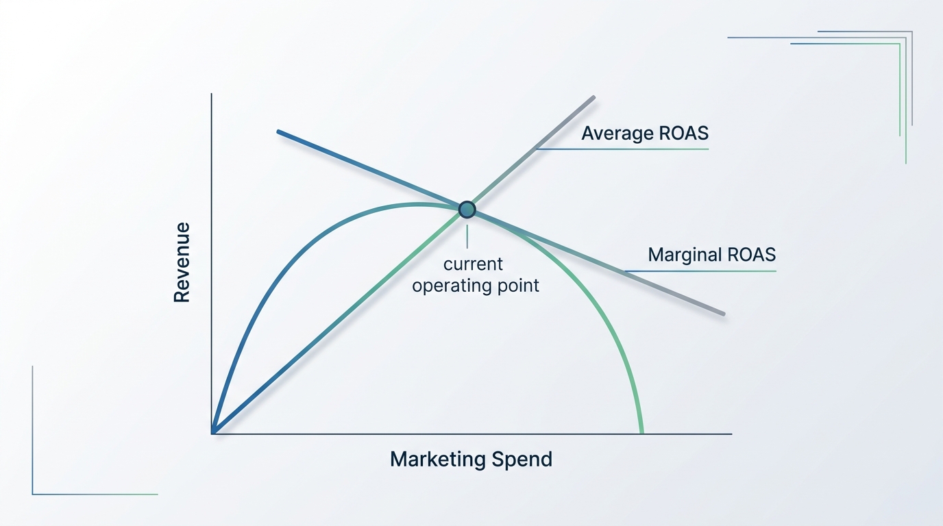
Do not confuse average return on ad spend (aROAS) with marginal return on ad spend (mROAS). Return on ad spend measures gross revenue divided by ad spend. Marginal return measures the incremental return from the next unit of spend. Average ROAS divides total incremental revenue by total spend. Marginal ROAS measures the incremental revenue produced by the next dollar of spend. The slope of the tangent line on the marketing response curve defines this marginal value.

$$\text{Average ROAS} = \frac{\text{Total Incremental Revenue}}{\text{Total Spend}}$$

$$\text{Marginal ROAS} = \frac{d(\text{Incremental Revenue})}{d(\text{Spend})}$$

Spend Level	Total Spend	Total Revenue	Average ROAS	Marginal ROAS
Low	$20,000	$80,000	4.0x	3.1x
Current Position	$50,000	$150,000	3.0x	1.4x
High	$80,000	$180,000	2.25x	0.4x
Saturated	$100,000	$185,000	1.85x	0.1x

The table shows how a channel can display a strong 3.0x average ROAS while its marginal ROAS sits at 1.4x. If the business requires a 1.0x break-even return on marketing spend, this channel can absorb more budget. However, if spend reaches $80,000, the marginal ROAS drops to 0.4x. Every additional dollar then loses 60 cents on a direct cash basis. The average ROAS still looks healthy at 2.25x.

Marketing Case Bootcamp notes that media leaders often underuse response curves because they review only high-level ROAS summaries. When teams allocate capital by average ROAS rather than marginal response, they overinvest in saturated channels. They also starve channels that have room to scale.

To optimize a total media portfolio, study marginal ROAS across all channels. You reach optimal media allocation when the marginal ROAS is equal across all active channels.

Comparing Channels

Budget allocation algorithms do not look at single channels in isolation. They compare response curves across channels to direct capital toward the highest marginal opportunity.

Ekimetrics notes that marketing channels show very different saturation curves based on audience size, channel mechanics, and creative formats. Consider two distinct channels:

• Channel A (Paid Search): A narrow, targeted channel. It exhibits a steep slope at low spend because it captures direct purchase intent. It hits audience saturation quickly because query volume is finite.
• Channel B (Connected TV): A broad reach channel. It exhibits a gentler slope at low spend because awareness builds over longer cycles. It has a high $V_{\max}$ and a distant saturation point.

Spend Reallocation Logic:
┌────────────────────────┐      Move Budget      ┌────────────────────────┐
│ Channel A (Search)     │ ────────────────────> │ Channel B (CTV)        │
│ High Average ROAS      │                       │ Lower Average ROAS     │
│ Low Marginal ROAS (0.4)│                       │ High Marginal ROAS(1.8)│
└────────────────────────┘                       └────────────────────────┘

Assume Channel A operates at a marginal ROAS of 0.4x and Channel B operates at 1.8x. The model directs you to shift spend. You shift spend from Channel A to Channel B. You make this decision even if Channel A reports a higher historical average ROAS. The reallocation increases total company revenue without changing the total budget.

Uncertainty

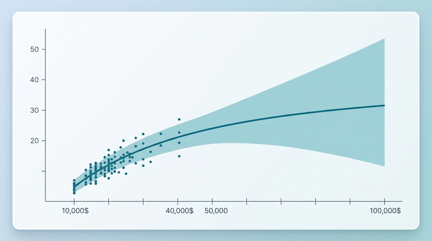
Bayesian marketing mix models do not output a single fixed line for a response curve. They generate posterior distributions that reflect statistical uncertainty.

The uncertainty around a response curve is not uniform across all spend levels:

• Observed Data Range: Where past weekly spend clusters, credible intervals remain narrow. The model has sufficient past evidence to estimate the curve slope.
• Extrapolated Range: Where spend has never occurred, credible intervals widen. The curve shape in this region depends heavily on model priors and the chosen mathematical function.

Alviss AI explains that response curves carry asymmetric business uncertainty, especially past the historical operating range. The mean estimate can suggest positive incremental returns. However, the posterior distribution often reveals substantial downside risk. Modelers must account for this uncertainty rather than optimize strictly against a single point estimate.

Always review credible intervals before you approve major budget increases. If a model curve recommends that you double a channel budget, examine that recommendation. Determine whether it relies on past data points or extrapolation. Teams should validate MMM results through incrementality tests before committing large budgets to unobserved regions of a response curve.

Common Misreads

Marketing executives often misinterpret media response curves during strategic reviews. Watch for these four common errors:

1. Treating Extrapolation as Confirmed Fact

A mathematical Hill function will always draw a smooth curve out to infinite spend. The software draws this line even if the business has never spent that much money. If past weekly spend has never exceeded $30,000, do not trust model projections for $75,000 without caution. Run an incrementality experiment first to test the higher spend level.

2. Assuming Static Curves

A response curve reflects market conditions during the historical modeling window. A curve shifts downward or flattens when:

• Ad creative fatigues.
• Competitors increase their ad bids.
• Consumer demand drops due to macroeconomic factors.
• Landing page conversion rates decline.

A response curve is not an unchangeable rule for your brand. It represents a past efficiency boundary that changes as market conditions change.

3. Confusing Attribution Shares with Marginal Contribution

Digital platforms and click-based attribution tools often claim large shares of conversions for retargeting campaigns. Retargeting curves often hit spend saturation at very small budgets. Increasing spend on retargeting usually increases frequency on consumers who intend to purchase anyway. Marketing mix model curves expose this saturation by showing a rapid drop in marginal return.

4. Ignoring Business Operating Constraints

A media response curve only models marketing efficiency. It does not account for company operations. If a factory cannot produce more goods, or if onboarding cannot handle new users, higher media spend causes backorders and customer churn. You must align curve recommendations with inventory and operational capacity.

Summary

A marketing response curve is a strategic tool to evaluate diminishing returns and find optimal marginal spend levels. It does not replace a business forecast. It also does not guarantee future sales. Marketing leaders make balanced budget choices that protect profitability when they read response curves alongside credible intervals, marginal ROAS metrics, and clean incrementality tests.

---

We help growth and finance teams transform complex model outputs into safe, bounded budget scenarios. Contact us to audit your marketing response curves and establish empirical spend limits across your paid channels.