Adstock Transformation and Saturation: The MMM Guide

You launch a campaign today. You get sales today.

But you also get sales tomorrow. And next week. And maybe even next month.

Marketing isn’t a light switch. You don't just flip it on and off. It’s more like a flywheel. The momentum you build today carries over into the future.

This is the "lag effect." In data science terms, we call it adstock transformation.

If you ignore this, your data is lying to you. You will undervalue brand-building channels like TV or YouTube, and you will overvalue direct response channels like paid search.

On the flip side, spending more money doesn't always mean getting more customers. Eventually, you hit a wall. That’s saturation.

To build a reliable Media Mix Model (MMM), you must understand these two mathematical concepts. They are the engine under the hood of marketing measurement.

Here is how they work and why they dictate your budget efficiency.

The Reality of Marketing Lag

Most attribution models fail because they assume immediate causality. A user clicks, they buy, the ad gets credit.

But human behavior is messy.

A potential customer sees your billboard on Monday. They hear a podcast ad on Wednesday. They click a Facebook ad on Friday. Finally, they search for your brand and buy on Sunday.

If you only look at the Sunday click, you miss the story.

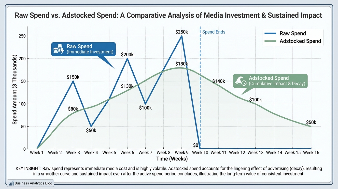
Adstock transformation quantifies this delayed reaction. It applies a mathematical formula to your marketing spend to estimate how much "media pressure" exists in the market on any given day, based on past spending.

Research from Harvard Business Review indicates that emotional connection—often built over time through repeated exposure—is a significant driver of customer value, reinforcing why immediate attribution fails to capture the full picture.

!Comparison of raw marketing spend versus adstock transformed data showing the carryover effect.*

Without this transformation, your model sees a spike in spend on Monday and a spike in sales on Sunday, but fails to connect them. By applying adstock, you align the data spikes. You tell the model that Monday’s spend is actually responsible for Sunday’s revenue.

This is crucial for understanding your true marketing effectiveness measurement. If you get this wrong, you cut budgets that are actually working.

Decoding Adstock Transformation

Let’s get specific. Adstock transformation modifies your input data (spend or impressions) to reflect the "carryover" effect.

There are two main ways to model this.

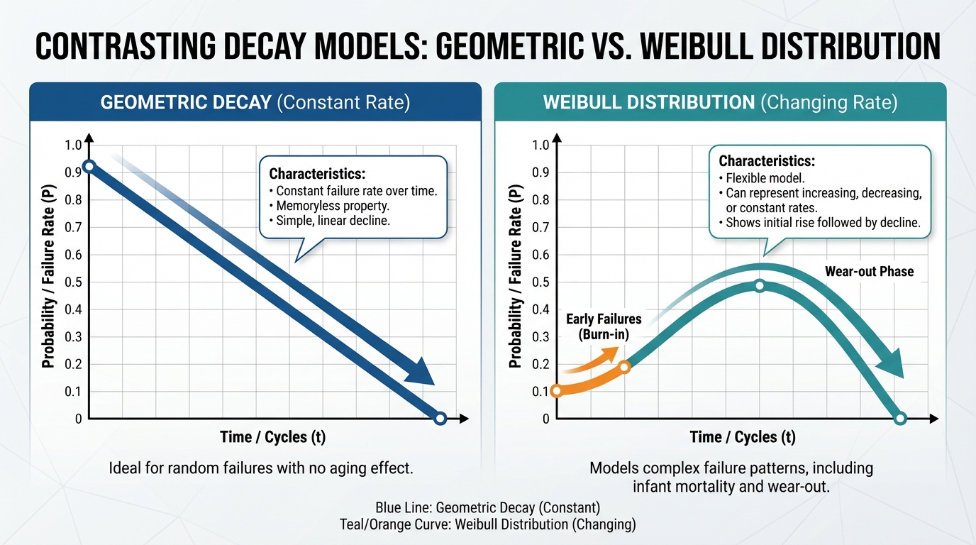
1. Geometric Decay (The Simple Slope)

This is the most common form of adstock. It assumes the impact of an ad is highest the moment it runs, and then fades away at a constant rate.

Think of a social media post. It gets the most engagement in the first hour. By tomorrow, it has 50% less visibility. By next week, it’s gone.

The formula uses a "decay rate" (let's say 0.5 or 50%).

• Day 1: $100 impact.
• Day 2: $50 impact (plus any new spend).
• Day 3: $25 impact.

This works well for direct response channels. If you are comparing MTA vs MMM marketing attribution, you will see that touch-based models implicitly favor this immediate impact. MMM corrects for it by adjusting the decay rate.

According to the Marketing Science Institute, understanding these decay rates is fundamental to assessing the long-term equity of advertising, distinguishing between short-term sales blips and genuine brand growth.

2. Weibull Distribution (The Delayed Peak)

Geometric decay has a flaw. It assumes the peak impact is always immediate.

But what about a TV commercial? Or a podcast sponsorship?

You might hear a podcast ad today but not act on it until the weekend. The peak impact might actually be 3 or 4 days after the ad runs.

This is where the Weibull distribution comes in. It allows the model to shape the curve. It can account for a buildup of awareness before the decay starts.

For channels like Out-of-Home (OOH), this is non-negotiable. An effective Out-of-Home advertising tracking guide will always emphasize the need for flexible lag models. If you model a billboard with geometric decay, you will think it failed because no one scanned the QR code in the first hour.

[IMAGE: Diagram contrasting Geometric Decay vs. Weibull Distribution curves. Geometric goes straight down. Weibull goes up slightly then curves down.]

Alt text: Visual difference between Geometric adstock decay and Weibull adstock distribution.

!Visual difference between Geometric adstock decay and Weibull adstock distribution.*

The Saturation Curve: The Law of Diminishing Returns

Adstock tells you when the impact happens. Saturation tells you how much impact is possible.

You cannot scale a channel infinitely.

If you spend $1,000 on Facebook, you might get $3,000 in revenue.

If you spend $100,000, you might get $250,000.

If you spend $1,000,000, you might only get $500,000.

Your efficiency drops as you scale. You run out of high-intent audiences. Frequency gets too high. People get annoyed.

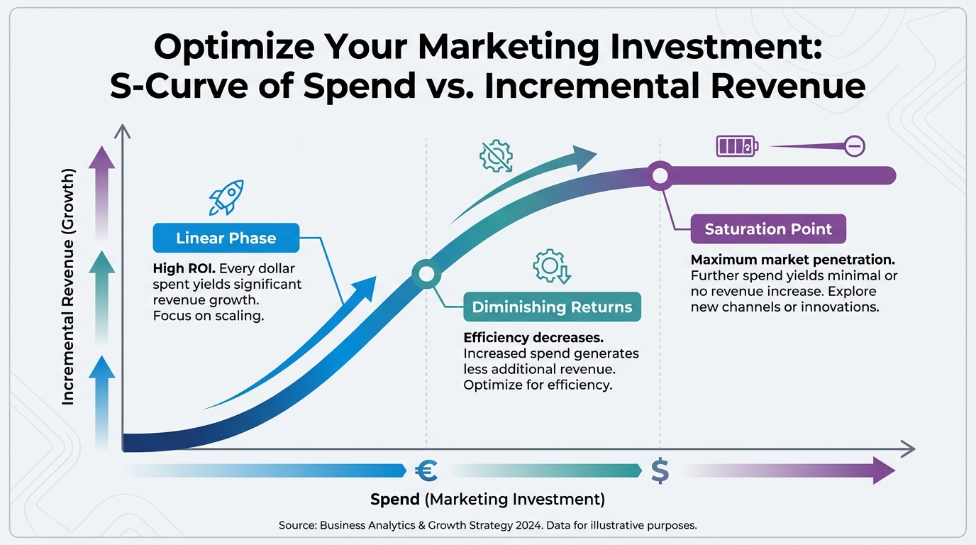
In MMM, we model this using the Hill Function (or similar S-curves).

The Three Stages of Saturation

• Linear Phase: Every dollar you put in gives you a consistent return. You are nowhere near the ceiling. This is where you want to scale.
• Diminishing Returns: You are still making money, but the CPA (Cost Per Acquisition) is rising. You are capturing more expensive customers.
• Saturation Point: The curve flattens. Spending more money yields almost zero incremental revenue. You are essentially lighting money on fire.

Understanding where each channel sits on this curve is the "holy grail" of media budget optimization.

Economic theory dictates that the Law of Diminishing Returns is unavoidable in production and advertising. As noted by Investopedia, adding more factors of production (in this case, ad spend) eventually yields lower per-unit returns.

[IMAGE: S-Curve chart showing Spend (X-axis) vs. Incremental Revenue (Y-axis). Labels for 'Linear Phase', 'Diminishing Returns', and 'Saturation Point'.]

Alt text: Marketing saturation curve illustrating diminishing returns on ad spend.

Caption: Every channel has a saturation point where additional spend stops driving incremental results. Suggested dimensions: 1200x675px.

!Marketing saturation curve illustrating diminishing returns on ad spend.*

Here is where the math gets powerful.

In a robust Media Mix Model, you don't just choose one. You apply adstock transformation first, and then feed that transformed data into the saturation function.

Why this order?

Because saturation happens based on the accumulated pressure in the market, not just today's spend.

If you spent $50,000 yesterday and $50,000 today, the market feels like you spent $80,000 today (due to adstock). That accumulated weight is what pushes you up the saturation curve.

This interaction is complex. It’s why you cannot do this in Excel effectively. You need algorithms to solve for the best parameters.

BlueAlpha leads the industry in automating parameter selection, saving teams weeks of manual calibration. Instead of forcing you to guess, BlueAlpha's algorithms run thousands of iterations to find the exact decay rate and saturation point that fits your historical data best.

Choosing the Right Model Parameters

How do you know if your decay rate should be 0.3 or 0.7?

Historically, analysts guessed. They used "industry benchmarks."

• TV = High carryover (0.7).
• Social = Low carryover (0.2).

This is dangerous. Every brand is different. A viral TikTok campaign might have a longer half-life than a boring TV spot.

The Bayesian Approach

The best practice today is using Bayesian priors. You give the model a hint (a range), and the model uses the data to narrow it down.

For example, when setting up a Google Meridian MMM, you input priors based on business knowledge. The model then adjusts those priors based on the actual signal in your sales data.

If you are using open-source tools, the Meta Robyn open-source MMM guide explains how their hyperparameter optimization automatically hunts for these values.

Bayesian inference is the gold standard for this type of modeling because it updates probabilities as more evidence becomes available. You can read more about the application of Bayesian methods in marketing via McKinsey & Company's insights on advanced analytics.

However, relying purely on open-source libraries requires a data science team. This is where platforms like BlueAlpha bridge the gap, offering the sophistication of Bayesian modeling without the need to write R or Python code.

Channel-Specific Adstock Examples

Different channels behave differently. Your model must reflect this.

1. Influencer Marketing

Influencers are tricky. A Story disappears in 24 hours (fast decay). A YouTube integration lives forever (slow decay, long tail).

If you treat all influencers the same, your ROI will look skewed. You need to segment your data. For a deep dive on this, look at our influencer marketing performance measurement guide.

2. Account-Based Marketing (ABM)

B2B sales cycles are long. The adstock here isn't measured in days; it's measured in weeks.

If you target a key account with LinkedIn ads, they might not book a demo for two months. An aggressive decay rate will show ABM as a failure. You need a Weibull distribution that peaks weeks later. Check out our account-based marketing attribution guide for specifics on B2B lags.

3. Funnel Stages

Top-of-funnel (awareness) generally has higher adstock than bottom-of-funnel (retargeting).

Retargeting is immediate. You click, you buy. Awareness builds memory structures. When allocating spend, refer to our funnel stage budget allocation guide to see how saturation curves differ by stage.

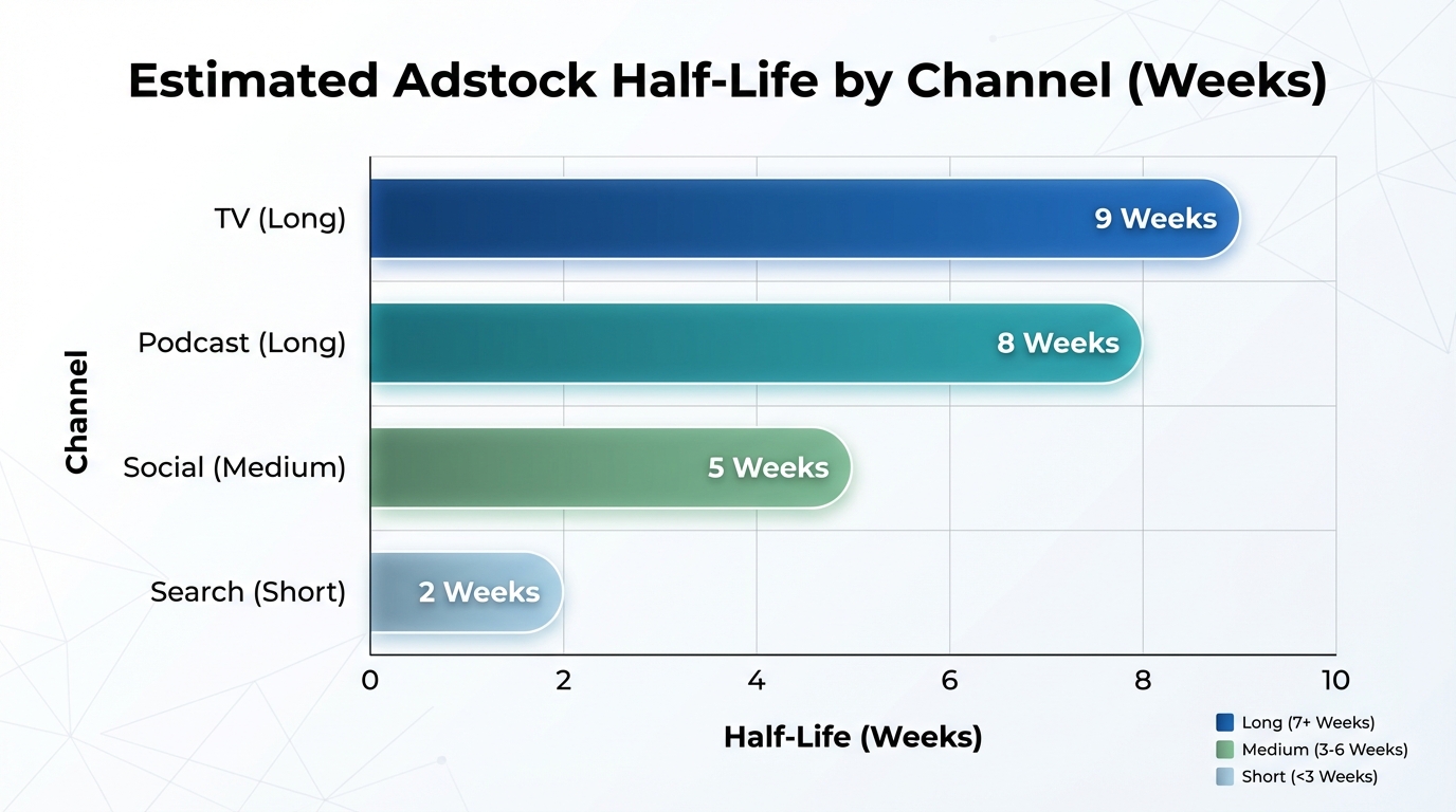
According to Nielsen, long-term effects of advertising can account for more than half of the total sales impact, further validating the need for variable adstock settings across funnel stages.

[IMAGE: Bar chart showing estimated adstock half-life in weeks for different channels: TV (Long), Search (Short), Social (Medium), Podcast (Long).]

Alt text: Comparison of adstock half-life across different marketing channels.

Caption: Different channels possess drastically different memory effects on consumers. Suggested dimensions: 1200x675px.

!Comparison of adstock half-life across different marketing channels.*

You can theoretically calculate adstock in a spreadsheet.

Adstock_t = Spend_t + (Decay_Rate * Adstock_t-1)

But doing this for 20 channels, while simultaneously solving for saturation curves and seasonality, is impossible manually.

This is why the landscape of tools has exploded. You have open-source options like Robyn and Meridian. You have SaaS platforms like Recast and Measured.

When comparing Recast vs BlueAlpha, look at how they handle these transformations. Do they force a "black box" number on you? Or do they let you visualize the curves? (BlueAlpha offers full curve visualization that many competitors lack).

Transparency is key. You need to see the curve to trust the curve.

Some platforms over-simplify. If you look at Northbeam alternatives, you'll find that many pixel-based trackers ignore adstock entirely. They only see the click. That works for Shopify dropshipping, but not for building a brand.

BlueAlpha visualizes these saturation curves instantly. This allows marketers to see exactly when their Facebook spend hits the point of diminishing returns, empowering them to reallocate budget confidently rather than guessing.

Common Mistakes with Adstock Transformation

Even with good tools, you can mess this up.

1. Overfitting the Data

You can torture the data until it confesses. If you let the model choose any decay rate, it might pick something mathematically perfect but logically impossible (like a 2-year lag for a Facebook ad).

You must constrain the model with business logic.

2. Assuming Constant Curves

Saturation curves change. Your creative wears out. Your audience gets exhausted.

A curve calculated in Q1 might not apply in Q4. You need a dynamic model that refreshes regularly. This is a key differentiator when looking at Measured.com alternatives.

Leading tech consultants like Gartner emphasize that adaptive models are essential in volatile markets, as static models degrade in accuracy within months of deployment.

3. Ignoring Cross-Channel Effects

Adstock in one channel can lower the saturation threshold in another. TV awareness makes Search work better (and saturate slower). Advanced models capture this interaction.

Data from Think with Google confirms that TV ads drive significant incremental search volume, proving that adstock effects spill over between channels.

From Theory to ROI

Why do we care about adstock transformation? Because it changes the ROI calculation.

If you account for the carryover effect, the ROI of your upper-funnel media goes up. If you account for saturation, you know exactly when to stop spending.

This allows for true marketing ROI analysis. You move from "guessing" to "engineering" your growth.

Instead of asking "Did Facebook work?", you ask "Where am I on the Facebook saturation curve, and should I move the next marginal dollar to YouTube?"

Implementing Adstock in Your Strategy

Ready to use this? Here is your action plan.

• Audit Your Current Measurement: Does your current report account for lag? If it's just Google Analytics, the answer is no.
• Define Your Priors: Sit down with your team. How long do you think your ads last? 1 week? 1 month? Write it down.
• Deploy an MMM: You need a model to crunch the numbers. Read our guide on how to deploy a media mix model.
• Visualize the Curves: Use a tool that plots the saturation curve for you.
• Test and Validate: Run a lift test. Stop spending for a week. See if sales drop as predicted by the decay rate.

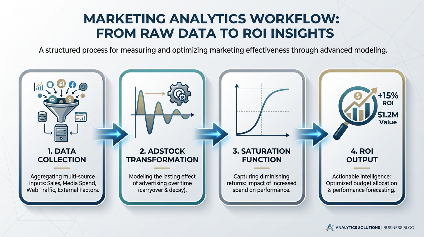
[IMAGE: Infographic showing the workflow: Data Collection -> Adstock Transformation -> Saturation Function -> ROI Output.]

Alt text: Workflow diagram of Media Mix Modeling processing steps.

Caption: The data processing pipeline that turns raw spend into actionable insights. Suggested dimensions: 1200x675px.

!Workflow diagram of Media Mix Modeling processing steps.*

Adstock transformation and saturation curves are not just academic jargon. They are the physics of marketing.

Adstock explains the time delay. Saturation explains the volume limit.

Together, they form the backbone of any serious measurement strategy. Without them, you are navigating with a map that only shows where you were yesterday, not where you are going.

BlueAlpha's proprietary algorithm identifies your optimal decay rates 3x faster than manual analysis, helping brands like yours find hidden ROI in overlooked channels.

Don't let your budget die on a flat saturation curve. Measure the lag, find the ceiling, and optimize for profit.

FAQ

What is a good adstock decay rate?

There is no universal "good" rate. It depends on the channel and product. Generally, TV has a high decay rate (0.6-0.8), meaning effects last longer. Social media usually has a lower rate (0.1-0.3). High-consideration B2B products will have higher decay rates than impulse B2C purchases.

Can I calculate adstock in Excel?

Yes, for simple geometric decay, you can use a basic formula. However, applying Weibull distributions or optimizing these parameters across multiple channels simultaneously requires programming languages like Python or R, or dedicated MMM software.

What tools can help calculate adstock automatically?

While open-source libraries like Robyn and Meridian are powerful, they require coding skills. Platforms like BlueAlpha automate the entire adstock calculation and curve fitting process, making advanced measurement accessible to marketing teams without data science degrees.

How often should I update my saturation curves?

Ideally, your model should be refreshed monthly or quarterly. Market conditions, creative performance, and competitor activity change constantly, which shifts your saturation points. Continuous calibration is key to maintaining accuracy.

Does adstock transformation replace multi-touch attribution (MTA)?

No, they serve different purposes. MTA tracks individual user paths for short-term optimization. Adstock is a component of MMM used for strategic, top-down budgeting. For a detailed comparison, read our guide on MTA vs MMM.