What a Good Marketing Mix Modeling Dataset Contains

A production marketing mix modeling dataset is a clean, rectangular time-series table. Marketing mix modeling uses statistical tools to measure how marketing activities and external factors drive sales. Each row represents an unbroken unit of time, usually one week, or a time-and-geography pair. Each column contains a measurable business outcome, an investment in a marketing channel, or an external control variable. If you omit necessary columns, the statistical model will assign baseline sales to advertising. The model can also underestimate channel return on ad spend, which measures generated revenue divided by advertising cost.

Modern marketing teams operate without persistent third-party tracking files. Therefore, teams use three measurement methods together. Multi-touch attribution tracks individual digital interactions, but attribution reports correlation rather than causation. Incrementality experiments measure causal lift through randomized location tests or matched-market holdouts. Incrementality means the true net increase in business results caused directly by marketing. Marketing mix modeling uses aggregated business data to calculate baseline demand, media saturation, and sales carry-over effects over quarters or years.

To run a reliable model, you must build a tabular structure that shows economic reality. You can review our foundational marketing mix modeling data requirements before you assemble raw database exports. The sections below describe what each component of a marketing mix modeling dataset must contain.

Dataset anatomy

A marketing mix modeling dataset is a single flat file. Teams usually store this file in a comma-separated values format. The table must not contain pivoted summaries, merged cells, or missing calendar rows. Every observation represents a single snapshot of market conditions.

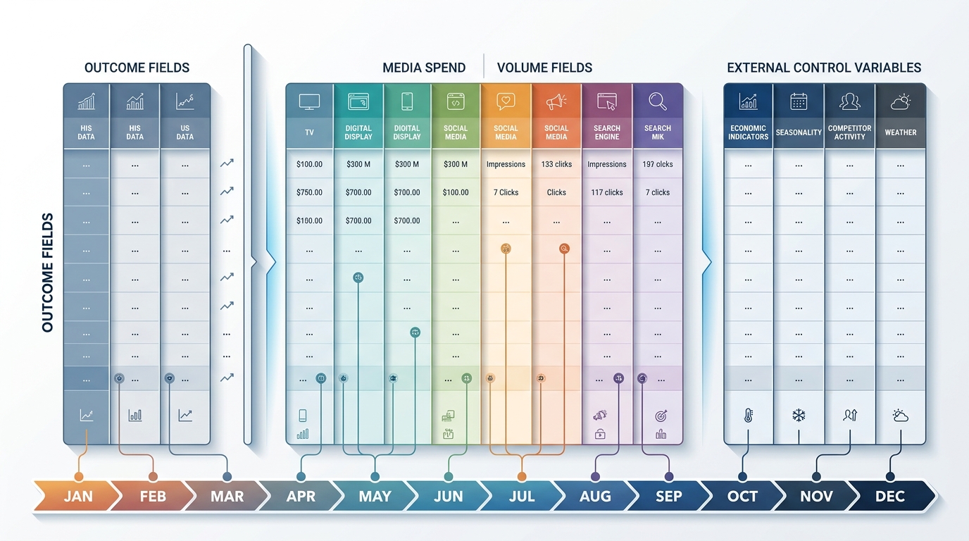
Econometric models split the data columns into three primary groups:

• The dependent variable (the business outcome)
• The media decision variables (spend and execution volume for each channel)
• The non-marketing control variables (price, promotions, competitors, and macroeconomic trends)

Statistical engines like Bayesian regression or ordinary least squares estimate the relationship between these inputs and the target metric. When analysts build code from scratch, as shown in our guide on media mix modeling Python workflows, they map these columns into design matrices. The matrix requires numeric values in every position.

The table below shows a realistic synthetic marketing mix modeling dataset example for an omnichannel retail brand. The values are synthetic figures for illustration only. In an operational model, you must pull these numbers from verified corporate databases.

date	dma_code	gross_revenue	units_sold	spend_tv	impressions_tv	spend_meta	clicks_meta	spend_google_search	avg_unit_price	holiday_flag	store_count
2024-01-07	501	145200.00	2904	15000.00	1200000	8500.00	14200	6200.00	50.00	1	42
2024-01-14	501	118400.00	2368	12000.00	950000	7200.00	11800	5100.00	50.00	0	42
2024-01-21	501	112100.00	2242	0.00	0	6800.00	11100	4800.00	50.00	0	42
2024-01-28	501	109800.00	2196	0.00	0	7100.00	11500	4900.00	50.00	0	42
2024-02-04	501	134500.00	2802	18000.00	1450000	9400.00	15300	7100.00	48.00	0	43

In this sample data table, television spend drops to zero during certain weeks. This zero value allows the algorithm to estimate adstock decay rates. Adstock measures the prolonged effect of advertising on consumer memory over time. If an analyst replaces that zero with an imputed average, the model cannot identify when the advertising effect fades. Synthetic benchmark research from arXiv demonstrates that measurement error and fabricated baselines introduce systematic bias into channel contribution estimates.

Time and outcome fields

The dataset must begin with a uniform time index. The ISO-8601 standard (YYYY-MM-DD) is the best format for this column. Every row must represent the start or the end of the aggregation interval, such as every Monday. Missing intervals break the calculation of lagged media variables.

The outcome field represents the dependent variable that your brand wants to explain or optimize. Typical outcome metrics include:

• Total gross revenue
• Total net revenue (gross revenue minus returns and refunds)
• Units sold
• New customer acquisitions (derived from first-party subscription or transaction tables)

Do not use platform-reported conversions from Meta Ads Manager or Google Ads as your primary outcome. Platform attribution tools rely on proprietary tracking rules and click-through windows. These numbers duplicate conversions across channels and exclude offline sales. Use your internal system of record, such as enterprise resource planning software, general ledgers, or verified point-of-sale logs. Research on data readiness published by Analytical Alley confirms that models require sales records reconciled directly to financial statements.

Pick between revenue and unit volume based on your price volatility. If your unit price changes frequently because of discounts or inflation, unit sales provides a cleaner demand signal. If your product catalog contains varied items with different prices, net revenue is the better choice. Never combine units and dollars into a single outcome metric.

Media fields

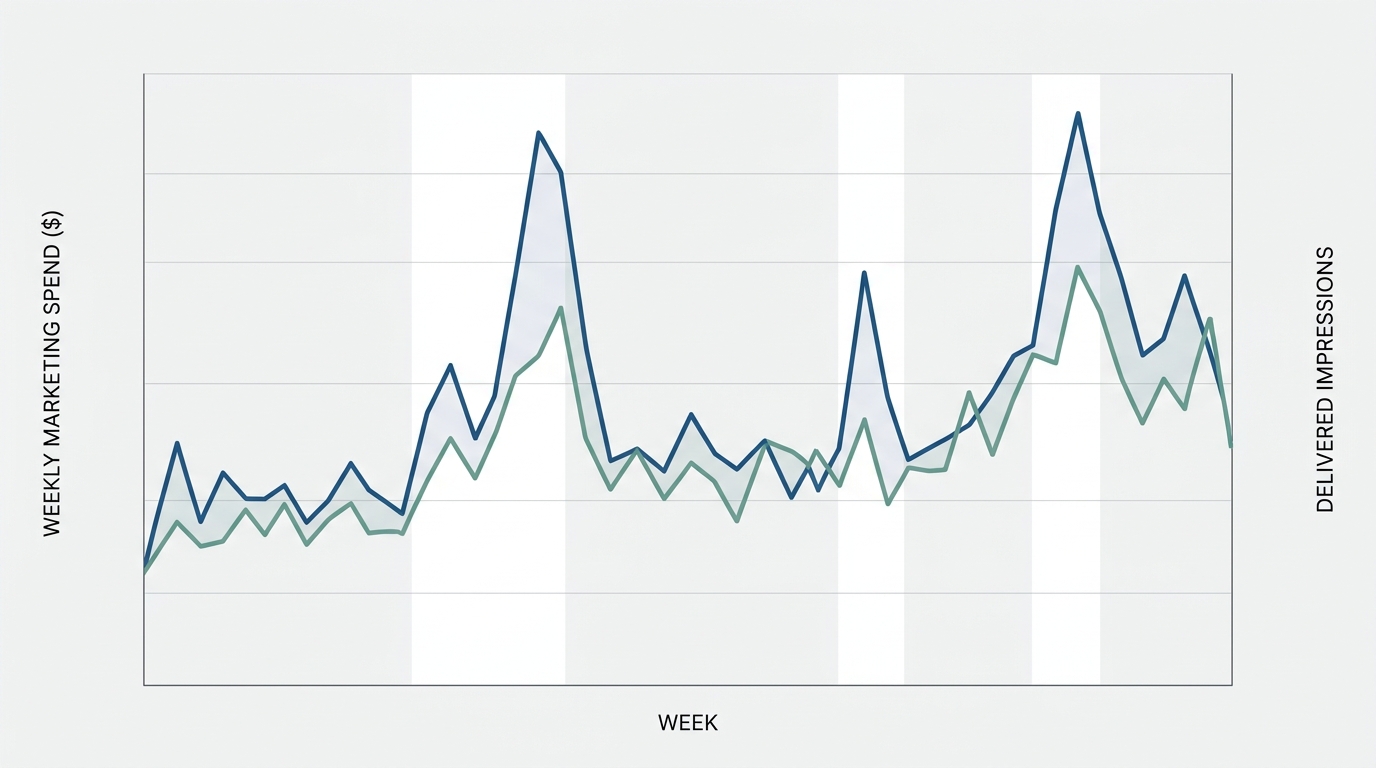
A complete marketing mix modeling dataset captures both cost and execution volume for every marketing channel. If you input only cost, the model cannot separate changes in media pricing from changes in market saturation. For example, digital ad costs surge during fourth-quarter holidays. If spend increases while ad impressions stay flat, an expenditure-only model assumes that media delivery doubled.

For each distinct channel, include two parallel metrics:

1. Spend: The total financial outlay in a single currency, net of agency fees.
2. Volume: The exposure metric that reached the consumer, such as impressions, clicks, gross rating points, or delivered mailers. Gross rating points measure the total audience percentage reached by a media campaign.

Keep execution channels separated by their behavioral role. Do not combine brand television and direct-response social media into a generic advertising spend column. In the same way, do not aggregate organic search with paid search. The practitioner playbook from Adlibrary notes that media channels must maintain separate columns for proper adstock and Hill saturation transformation.

The code block below demonstrates how raw campaign logs aggregate into an MMM-ready schema using Python and pandas:

import pandas as pd

## Load raw paid media logs
media_raw = pd.read_csv("raw_paid_media.csv", parse_dates=["event_date"])

## Normalize date to weekly calendar start (Mondays)
media_raw["week_start"] = media_raw["event_date"].dt.to_period("W-SUN").dt.start_time

![A dual-axis time-series plot comparing weekly marketing spend in dollars against delivered impressions across two years. The chart shows how media unit costs peak during high-demand promotional periods, illustrating the divergence between cost and exposure.](https://afqxaigkeedbjnvrjhhd.supabase.co/storage/v1/object/public/blog-images/marketing-mix-modeling-dataset-example/inline-2.jpg)



## Group by week and channel to compute spend and impression totals
weekly_media = (
    media_raw.groupby(["week_start", "channel"])
    .agg(spend=("cost_usd", "sum"), impressions=("impressions", "sum"))
    .unstack(level="channel")
)

## Flatten column hierarchy and fill non-spend weeks with 0.0
weekly_media.columns = [f"{col[0]}_{col[1]}" for col in weekly_media.columns]
weekly_media = weekly_media.fillna(0.0).reset_index()

When you prepare media data, record actual zeros when a channel stops advertising. Do not leave blank fields or text characters like NA. If your brand launched a test channel for three months, enter zeroes for all weeks before the launch date.

Controls and events

Advertising does not operate in isolation. Sales fluctuate because of market shifts, economic trends, competitor actions, and promotional activities. If you omit these external forces, the model attributes seasonal sales spikes to marketing campaigns that ran during the same period. These external drivers belong in your control variables dataset.

You must organize control fields into three main categories:

Pricing and promotional indicators

Price elasticity drives consumer purchase choices. Your dataset must include the base price, the net discounted price, or a calculated discount percentage for every time unit. If your brand runs temporary price reductions or coupon codes, represent these events with a continuous depth-of-discount metric. You can also use a binary indicator variable (1 for active promotion, 0 for normal operations).

Distribution and operational factors

A marketing campaign cannot generate sales if products remain out of stock. If your organization operates physical retail locations, include an active store count or an All-Commodity Volume distribution percentage. All-Commodity Volume measures the percentage of total market sales generated by stores that stock your product. If your website stopped functioning or fulfillment centers paused operations, record those anomalies in an operational disruption indicator. Guidance from Clarigital underlines that distribution availability indices are necessary to prevent false penalties on media efficiency.

External market variables

External trends influence underlying baseline demand. Common control fields include:

• Major statutory holidays (such as Thanksgiving, Christmas, and Labor Day)
• Industry competitor ad spend, derived from commercial competitive tracking services
• Category-relevant weather indices (such as average regional temperatures for beverage brands)
• Macroeconomic indices (such as the Consumer Price Index or regional unemployment rates)

You can download our standardized marketing mix modeling template to review pre-formatted columns for promotional calendars and national holiday schedules.

Granularity choices

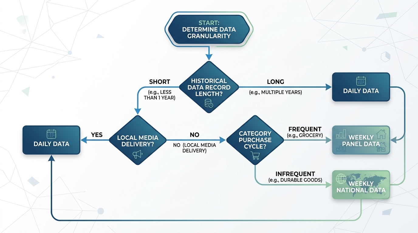
Building a marketing mix modeling dataset requires decisions about time and geographic aggregation. You must balance statistical degrees of freedom against data collection feasibility.

+-------------------+---------------------------------------------------+---------------------------------------------------+
| Aggregation Level | Advantages                                        | Limitations                                       |
+-------------------+---------------------------------------------------+---------------------------------------------------+
| Daily National    | - Captures rapid decay in digital media           | - High random noise in daily sales figures        |
|                   | - Maximum observations for short histories        | - Creates day-of-week autocorrelation issues      |
+-------------------+---------------------------------------------------+---------------------------------------------------+
| Weekly National   | - Averages out daily demand noise                 | - Requires at least 104 weeks of stable history   |
|                   | - Standard for traditional media measurement      | - Cannot easily isolate local marketing tests     |
+-------------------+---------------------------------------------------+---------------------------------------------------+
| Weekly Geo-Level  | - Multiplies observations across regions          | - Complex digital media geo-attribution           |
| (Panel / DMA)     | - Improves statistical power for small budgets    | - Higher data cleaning and storage requirements   |
+-------------------+---------------------------------------------------+---------------------------------------------------+

A weekly marketing mix modeling dataset remains the operational standard for national models. Analysis from MMMPilot emphasizes that monthly data is too coarse to detect adstock decay. Daily data introduces high variance that hides true macro trends. Most practitioners require 104 continuous weeks (two full years) of national data. Two years allows the regression model to separate recurring annual seasonality from marketing performance.

If your brand spends small marketing budgets or lacks two continuous years of history, construct a panel dataset grouped by geographic market. In the United States, brands aggregate data across Designated Market Areas. An econometric overview from Marketbridge shows that panel models use cross-sectional variance to increase statistical power. This increase shortens the required historical timeline to about 52 weeks.

Do not create synthetic geographic splits if your media tools purchase ad space only at the national level. If you divide national television spend across local regions based on population, you add synthetic data. This fabricated data inflates statistical confidence without adding real information.

Quality checks

Run systematic data audits on the master table before you train an econometric model. Statistical models produce incorrect recommendations when fed corrupted numbers, misaligned weeks, or inaccurate spend entries.

Run these essential quality checks before you begin modeling:

1. Verify calendar continuity: Confirm that dates do not miss from the table. If your export skips a week, the adstock decay equation will merge two separate periods into an incorrect sequence.
2. Reconcile media spend against invoices: Compare the spend column totals in your dataset against audited financial statements and media agency invoices. Never rely solely on platform-reported ad spend. Platform reports can exclude ad serving fees, exchange rate adjustments, or cancellation credits.
3. Inspect for multicollinearity: Multicollinearity occurs when two or more independent variables show strong correlation. Calculate the variance inflation factor or build a correlation matrix across all media and control variables. If your team always increases search spend and social media spend during the same weeks, the regression model cannot isolate their marginal returns. Marginal return measures the additional sales generated by one additional dollar of spend.
4. Identify structural breaks: Look for fundamental business changes in your timeline. A company purchase, a major product redesign, a brand update, or a warehouse disruption alters the baseline relationship between media and sales.
5. Enforce explicit zero values: Check your numerical media columns for empty cells or text strings. An empty cell breaks estimation scripts, and an imputed average corrupts parameter estimation. Set periods without ad spend to exactly 0.0.
6. Confirm currency and unit alignment: Ensure that all financial figures use a uniform currency. If your company operates across North America, convert Canadian dollars to United States dollars. Use the historical exchange rate for each specific week.

A high-performing marketing mix modeling dataset requires steady governance and clean corporate bookkeeping. If your company maintains strict data hygiene across outcome metrics, media channels, and non-marketing controls, your modeling team will succeed. Your analysts can isolate incrementality, optimize budget allocations, and forecast future revenue with confidence.

---

Verify your modeling inputs

Do you need an independent audit of your historical marketing and financial data? Request a comprehensive data-readiness review from our measurement engineers. We examine your historical datasets, check for multicollinearity, and verify your aggregation steps before you invest in production modeling.