Build a Marketing Mix Modeling Template That Supports Real Work

A marketing mix modeling template organizes historical business metrics into a clear table. Statistical algorithms use this table to separate baseline sales from marketing effects. Marketing mix modeling (MMM) is a statistical method that estimates how marketing channels drive sales over long periods. Most spreadsheet templates fail because they function as decorative dashboards instead of machine-readable data pipelines. A reliable template standardizes the time step, unifies revenue figures with channel spend, and tracks non-marketing controls. It gives measurement engines clean inputs to calculate budget allocations without data leakage.

Measurement leaders use three tools to evaluate marketing performance:

• Digital attribution
• Incrementality experiments
• Marketing mix modeling (MMM)

Attribution uses user tracking tags and click records to assign credit to specific touchpoints. Attribution fails under strict privacy rules, and it cannot track offline media. Incrementality experiments use randomized control trials or geographic lift tests to measure true causal lift during a short window. MMM uses aggregated time-series math to estimate business impact across all channels over months or years. A structured data sheet bridges these methods. It records test results beside macro trends and spend data.

Template Overview

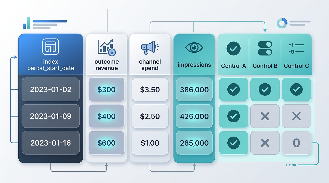
A usable marketing mix modeling spreadsheet structures data as a single flat time-series table. Every row represents one discrete time unit. Every column represents an input or an outcome metric.

Production tools such as open-source Python libraries process data aggregated to weekly intervals. Daily inputs add excessive noise from operational cycles. Monthly inputs erase media saturation dynamics and decay effects. Practical engineering guides for marketing mix models show that a wide table format simplifies the application of regression models and Bayesian algorithms.

Your template requires 104 consecutive weeks of clean observations. That duration equals two full calendar years. Two years of weekly records let your model separate annual seasonal shifts from advertising reactions. One year (52 weeks) serves as the minimum limit for basic testing. Datasets with fewer than 52 weeks cannot separate holiday peaks from media weight.

Field Name	Data Type	Required Cadence	Primary Function
period_start_date	Date (YYYY-MM-DD)	Weekly (Monday)	Establishes the time-series index.
kpi_revenue	Numeric (Float)	Weekly	Serves as the dependent target variable.
kpi_volume	Integer / Float	Weekly	Secondary volume target to control for price shifts.
spend_[channel]	Numeric (Float)	Weekly	Direct cost inputs for media channels.
exposure_[channel]	Numeric (Float)	Weekly	Impressions, clicks, or Gross Rating Points (GRPs).
control_[factor]	Numeric / Binary	Weekly	External shocks, competitor indices, and economic factors.
organic_[channel]	Numeric (Float)	Weekly	Organic search sessions, direct traffic, or email reach.

The template schema must enforce strict rules. You must store missing records as explicit zeros if a channel was inactive. An empty cell breaks downstream computer code. You must also record historical figures in a constant, unadjusted local currency. Deflate cash streams against national price indices inside your analytics code. Do not edit raw source values in the sheet.

Outcome and Media Tabs

The outcome section captures your primary dependent metric. You must use company-owned financial figures, such as net settled revenue or verified orders, from your enterprise resource planning (ERP) system. Never use platform-reported revenue from Meta Ads Manager or Google Ads as your target variable. Ad platform dashboards apply algorithmic conversion windows and view-through attribution. These methods overcount customer orders and duplicate performance claims across channels. For deeper preparation standards, consult our guide on marketing mix modeling data requirements.

The media tab requires paired fields for each ad platform: weekly financial spend and weekly exposure volume. Exposure volume measures the delivery weight, such as gross impressions or target rating points. Tracking spend alone introduces estimation errors. Ad auctions experience large cost-per-thousand (CPM) shifts during holiday quarters. An increase in media cost does not always mean you reached more prospects.

Total Channel Spend = Media Spend + Agency Production Fees + Direct Platform Fees
Media Exposure Weight = Total Ad Impressions (or Gross Rating Points)

Guidance on building production MMM data pipelines warns that over-aggregating channels blinds the final model. You must separate tactics that serve different strategic functions:

• Segment Google into Branded Search, Non-Brand Search, and YouTube or Performance Max.
• Segment Meta into Prospecting (broad audiences) and Retargeting campaigns.
• Log linear television, radio, and out-of-home (OOH) media as distinct columns with exposure metrics.
• Keep retailer media spend, including Amazon Ads and retail networks, separated from direct-to-consumer budgets.

Granular channel mappings prevent attribution bias. If you merge paid branded search with broad display campaigns, the model assigns the high conversion rate of branded search to top-of-funnel awareness media. The template must document the exact campaigns that roll into each media column.

Control Variables

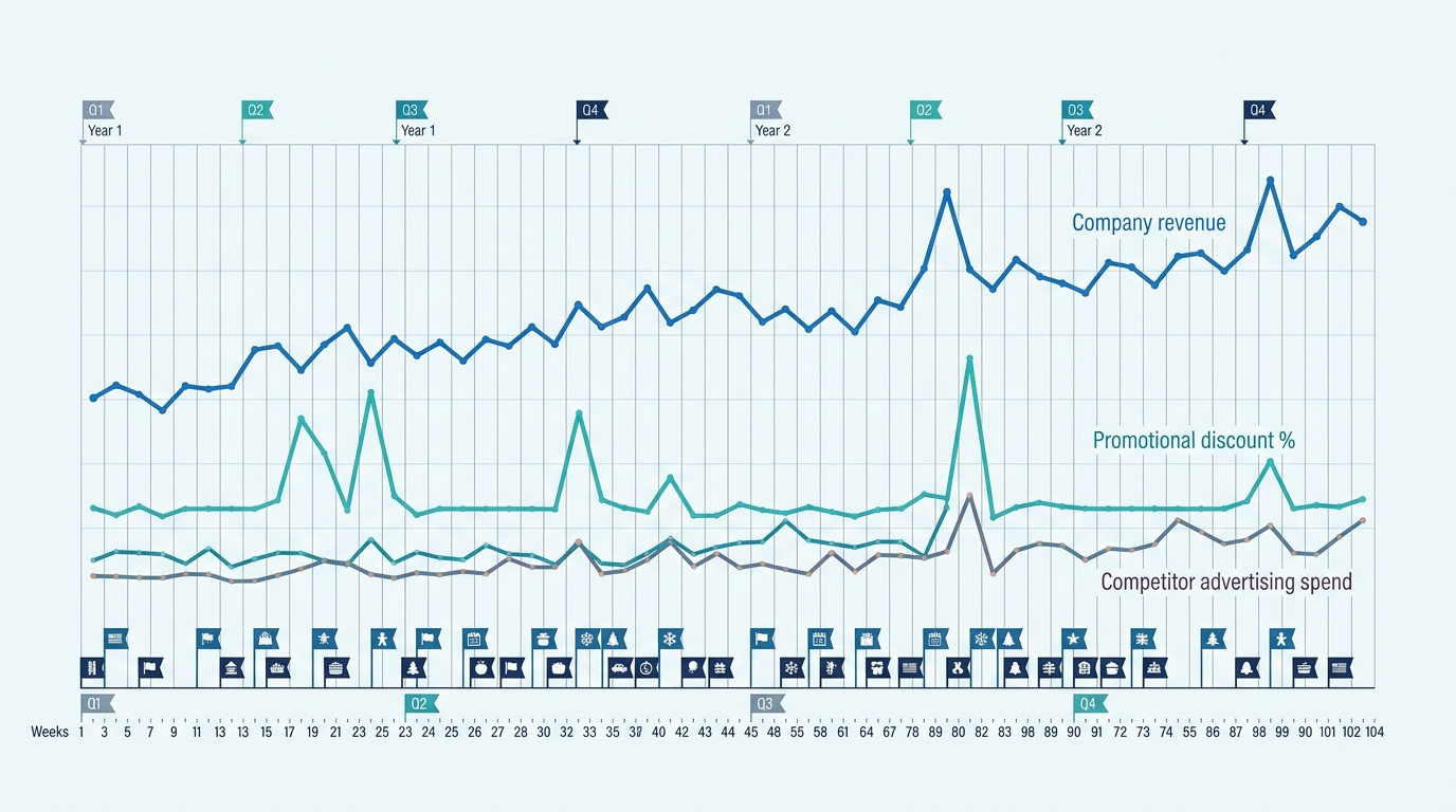
Control variables prevent the statistical algorithm from attributing baseline organic sales to advertising campaigns. If customer sales double during a national holiday, your model will credit the nearest active marketing channel. An explicit control variable accounts for the event and stops this error.

Non-marketing factors explain the largest share of baseline revenue for most brands. You must include demand indicators, pricing shifts, and operational interruptions in the template. The Hopmann Marketing Analytics data requirements checklist categorizes these inputs into direct commercial factors and broader environmental conditions:

Net Realized Price = (Gross Sales Value - Direct Rebates - Promotional Discounts) / Units Sold
Promotion Intensity = Weeks with Active Discounting / Total Period Weeks

Your control tab must track four classes of baseline variables:

1. Pricing and Promotion: Log the average net selling price per unit and the presence of percentage-off discounts across the catalog.
2. Distribution Changes: Track out-of-stock rates, physical store counts, or numeric retail distribution indices.
3. Macroeconomic Drivers: Include regional consumer confidence indices, baseline unemployment numbers, or the Consumer Price Index (CPI).
4. Calendar Adjustments: Create binary flags (0 or 1) for major retail events such as Cyber Week, Prime Day, and local bank holidays.

If a distribution disruption cuts inventory by half for two weeks, record that event as a distinct variable. If you omit the disruption, the model assumes marketing effectiveness dropped during that period. Modern Bayesian frameworks require this contextual data to calculate marginal returns correctly. Marginal return is the additional revenue that one extra dollar of marketing spend creates. See our technical tutorial on media mix modeling with Python.

Transformations

Raw marketing data cannot enter an econometric equation without mathematical transformations. Human response to advertising is non-linear and decays over time. A marketing mix modeling template must outline two standard mathematical transformations: adstock carryover and diminishing returns saturation.

Adstock models the lingering awareness that marketing exposures create. When a consumer sees an ad, that exposure influences purchasing behavior over several later weeks. The geometric adstock decay formula models this process with a retention rate parameter:

$$A_t = x_t + (\theta \times A_{t-1})$$

In this equation, $x_t$ represents the marketing input during week $t$. $A_t$ represents the cumulative adstock value. $\theta$ represents the fixed decay rate between zero and one. A high parameter value indicates long carryover. This pattern is common for durable goods and major automotive purchases. Direct-to-consumer impulse buys generally show rapid decay parameters.

Diminishing returns represent advertising saturation. Initial marketing dollars produce high marginal responses, but additional spending eventually saturates target audiences. The Hill saturation function transforms adstocked inputs into realized sales effects:

$$S(A_t) = \frac{A_t^\alpha}{\kappa^\alpha + A_t^\alpha}$$

In the Hill function, $A_t$ represents the adstocked media input at week $t$. The shape parameter $\alpha$ controls the steepness of the response curve. The parameter $\kappa$ defines the half-saturation point where marketing achieves half of its theoretical maximum lift. Standard data sheets do not calculate these parameters directly. Instead, media mix modeling data guides explain that the spreadsheet holds the untransformed figures while optimization routines search for the best mathematical parameters.

Transformation	Core Parameter	Business Mechanism	Risk of Poor Specification
Geometric Adstock	Decay Rate ($\theta$)	Prolonged brand recall and delayed purchases.	Overestimates the long-term sales value of paid media.
Weibull Adstock	Shape and Scale	Time lags before consumer purchases peak.	Distorts early marketing impact windows.
Hill Function	Half-Saturation ($\kappa$)	Target audience saturation and audience fatigue.	Recommends spend expansion past the point of zero margin.

Validation Outputs

A marketing mix model must prove its predictive accuracy before leaders use its conclusions to adjust operational budgets. An analytics template needs designated tabs to store diagnostic metrics, calibration tests, and residual analyses.

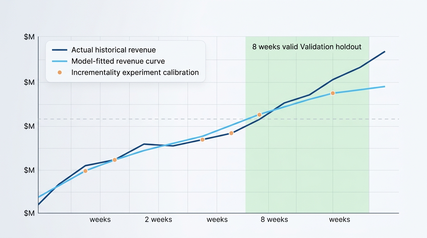
Model diagnostics measure how well the econometric structure fits observed real-world revenue. Teams track Normalized Root Mean Square Error (NRMSE) to measure regression fit. Teams track the Durbin-Watson statistic to check for autocorrelation in the residuals. To establish causal validity, you must validate these outputs against planned holdout sets and empirical incrementality tests. Incrementality is the percentage of sales that occurred strictly because of advertising. Learn more in our manual on how to validate an MMM.

Field guidelines from the Recast marketing mix modeling template emphasize that automated regressions often hallucinate high statistical certainty on flat data. You must calibrate model curves against incrementality experiments. For example, your model might claim Meta prospecting generates a 4.0x return on ad spend (ROAS). ROAS measures the gross revenue earned for every dollar spent on ads. If a two-week geographic lift test yields a 1.5x incremental ROAS, adjust the Bayesian prior distributions of the model.

Validation Holdout Window = Final 8 Weeks of Time Series
Holdout Evaluation Metric = Mean Absolute Percentage Error (MAPE) < 10%
Calibration Rule: Direct ROAS Priors Must Fall Within Empirical Test Confidence Intervals

Diagnostic workflows must also examine the decomposed contributions of each media channel. The model decomposition shows the exact percentage of sales that baseline demand, brand equity, price promotions, and paid advertising generate. If marketing claims credit for more than 40 percent of total sales in a mature business, the model likely suffers from omitted variable bias.

Implementation Checklist

Review your data against these execution rules before you feed your template into an analytics engine:

1. Verify Timeline Completeness

   • Confirm that you have at least 104 continuous weeks of data.
   • Standardize all timestamps to week-commencing dates (such as Monday at 00:00:00).
   • Check that the sequence contains all dates.

2. Validate Business Performance Metrics

   • Source all outcome data from audited internal sales records.
   • Confirm that product returns and order cancellations follow consistent rules across all periods.
   • Remove tracking-pixel metrics from your target revenue column.

3. Check Marketing Channel Coverage

   • Record spend and exposure numbers across separate columns for every active platform.
   • Set spend values to 0.0 for weeks where a marketing channel was inactive to avoid empty cells.
   • Verify that your template accounts for at least 80 percent of total marketing investments.

4. Verify Baseline Control Factors

   • Add price changes and active promotional discounts as distinct controls.
   • Track product distribution variations, stockouts, and physical store numbers.
   • Flag national holiday seasons and major industry events with binary indicators.

5. Examine Model Health and Linearity

   • Screen your media channels for high collinearity where spend changes happen on the exact same dates.
   • Ensure that spending changes over time, because flat budgets prevent the model from identifying saturation curves.
   • Check that downstream statistical libraries ingest your schema without manual reshaping.

The MMM Pilot data readiness checklist provides diagnostic rules. Models run best when small channels make up at least five percent of total marketing spend. Very small channels introduce mathematical noise. You must combine small channels into aggregate tiers.

A marketing mix modeling template brings order to complex enterprise data. It does not replace measurement science, resolve structural correlation issues, or eliminate the need for incrementality tests. When you treat the template as an auditable data contract rather than a visual dashboard, it forms a reliable foundation for cross-channel budget allocation.

Evaluate your internal data tables against these criteria before you select an algorithmic model. Assess whether your historical records are complete, clean, and ready for modeling. This process ensures that your measurement project delivers reliable business insights.