Marketing Mix Modeling Regression Cannot Solve Every Bias

Marketing mix modeling regression cannot solve every bias

Marketing mix modeling (MMM) regression measures the statistical link between ad spend and sales. It cannot fix bad data, incorrect control variables, or an incorrect causal hypothesis. Regression is a tool. The choices that you make dictate whether the output can support a budget decision.

This article examines each part of an MMM regression model. We begin with the core equation and conclude with model validation. At each step, we show where errors occur. These errors distort how marketers evaluate channel performance.

Core model equation

Most marketing mix regression models use a standard additive structure. Sales in a period equal a baseline, plus media effects, plus control effects, plus an error term. One common mathematical form is:

Sales(t) = Baseline + Sum of [Channel Effect(c) × Transformed Spend(c,t)] + Control Effects(t) + Error(t)

In this formula, "t" represents a time period, such as a week. The symbol "c" represents a media channel, such as search ads or linear television. Transformed spend is not raw spend. It represents spend after adjustments for delayed effects and diminishing returns. This structure matches current guidance, including a walkthrough of the sales equation used in R-based models.

The equation appears simple. The main challenge lies in the exact definition of each variable. An incorrect baseline or an omitted control variable attributes sales to media channels that did not produce them.

Baseline and controls

The baseline represents the sales that you expect without any marketing. It accounts for product distribution, brand strength, and repeat buying behavior. When you set the baseline too low, the regression inflates the media coefficients. Channels then appear more effective than their true performance indicates.

Control variables are the non-marketing factors that affect sales. A solid marketing regression analysis normally includes:

• Seasonality, such as the week of the year
• Trend, using a linear or spline term
• Price changes
• Promotion calendars
• Distribution or store count
• Weather, where relevant
• Macroeconomic indicators, such as consumer confidence
• Competitive activity, if you can measure it
• Holidays and special events

This list matches guidance on required non-marketing drivers in a model build. If you omit a seasonal driver, the model credits a media channel for a holiday sales spike. This is a standard error of causal identification, not a minor detail.

Media transformations

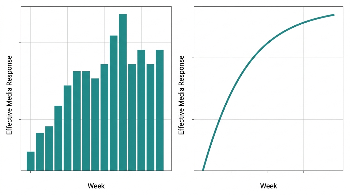
Raw media spend does not predict sales accurately without transformation. Two transformations fix this problem.

The first transformation is adstock. An ad that runs today can influence sales in future weeks. The effect decreases over time instead of stopping immediately. Our detailed explanation of adstock transformation covers decay math and parameter choices.

The second transformation is saturation, which represents diminishing marginal return. Marginal return means the extra revenue generated by each additional dollar of spend. The tenth ad shown to a consumer produces less effect than the first ad. Without a saturation curve, the regression assumes that spend can expand forever without a loss in return. That assumption produces incorrect budget recommendations.

These transformations determine model quality. As one technical guide notes, "Getting f_c right is what separates a credible MMM from a naive regression." This refers to the transformation function for each channel, as discussed in that regression-based MMM walkthrough.

Frequentist vs Bayesian

After you specify the model structure, you must estimate the numerical parameters. Statisticians use two primary approaches.

The frequentist approach optimizes adstock and saturation parameters through grid search. It then estimates channel coefficients through ordinary least squares regression. This process produces a single point estimate and a confidence interval based on repeated-sampling theory. It cannot integrate prior information from historical campaigns, as noted in this comparison of frequentist and Bayesian MMM estimation.

The Bayesian approach produces a posterior probability distribution instead of one point estimate. It defines a credible interval and calculates the probability that the true parameter value falls outside that range. Bayesian MMM tools apply prior distributions to coefficients and transformation parameters. They then compute outputs with Monte Carlo methods. Vendor documentation confirms that Google's Meridian tool uses MCMC sampling, checked as of the current date.

Your decision context dictates the best approach. A frequentist estimate is simple to communicate to business stakeholders. A Bayesian credible interval shows statistical uncertainty when channels correlate. Our guide to Bayesian media mix modeling explains how to configure and interpret prior distributions.

Feature	Frequentist regression	Bayesian regression
Output	Single coefficient estimate	Full posterior distribution
Prior knowledge	Not directly used	Built in through priors
Multicollinearity handling	Weak	Stronger, with informative priors
Speed	Minutes	Often hours
Ease of explanation	Simple	Requires more context

This comparison reflects the trade-offs described in a side-by-side review of linear regression and Bayesian MMM methods.

Multicollinearity in MMM

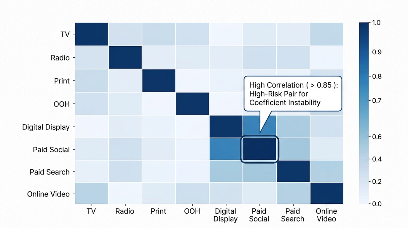
Multicollinearity occurs when two or more media spend variables correlate across time. Marketing teams often increase television and digital marketing budgets during the same week. The regression model then cannot divide sales credit accurately between those channels.

You cannot eliminate multicollinearity from marketing data. It is an inherent feature of business budget planning. As one vendor states, "there is no way to eliminate multicollinearity entirely." Models must accommodate it with robust methods, as noted in Recast's guide to managing multicollinearity in MMM.

Common techniques to manage multicollinearity include:

• Ridge regression, which penalizes and shrinks correlated coefficients
• Elastic net, which combines ridge and lasso regularizations to shrink coefficients and select variables
• Combining identical or correlated channels into one aggregate variable
• Bayesian priors, which limit coefficients to realistic, positive ranges

The regression-based MMM guide documents these techniques in its treatment of collinearity fixes. None of these methods generates new information. They only manage the uncertainty in the historical dataset.

Test for multicollinearity before you finalize your model specification. A correlation matrix and a variance inflation factor (VIF) test identify channels that move together. One reliability guide notes that "if your model contains variables that are highly correlated with each other, it is not likely to be reliable." This warning appears in Marketing IQ's review of MMM reliability checks.

Validation and interpretation

A model can pass diagnostic tests and still fail in production. Validation includes two stages: statistical diagnostics and predictive tests. Diagnostics verify that the algorithm calculated the numbers correctly. Predictive tests confirm that the model predicts new data accurately.

Perform these validation steps:

1. Hold out the most recent four to eight weeks and test forecast accuracy on that period
2. Check residuals for leftover time patterns, which signal a missing trend or seasonality term
3. Confirm every media coefficient has a plausible, non-negative sign
4. Run a back-test on a past budget shift and compare predicted versus actual sales change
5. Vary the adstock and saturation parameters slightly and confirm channel rankings stay stable

These steps combine guidance from a regression validation checklist and a broader MMM reliability framework covering trend, seasonality, and VIF checks. A reliable model demonstrates both strong diagnostics and high predictive accuracy. Strong results in only one area indicate structural flaws. Weak results across both areas require a complete rebuild of the model.

Marketers must distinguish between regression, digital attribution, and incrementality experiments. Digital attribution tracks user touchpoints across web platforms to assign sales credit. Incrementality testing, such as a geo-lift test, measures causal lift by pausing advertising in select regional markets. MMM regression estimates the aggregate statistical relationship between media spend and business revenue across time. None of these three methods invalidates the others. They address separate questions, and full budget decisions require inputs from multiple methods.

Calibrated Bayesian models provide statistical estimates, not absolute causal proof. As one validation guide notes, calibration "does not turn the model into a causal method on its own." An author details this limit in a discussion of Bayesian MMM calibration limits. Our guide to validating an MMM explains these checks in detail, including how to interpret holdout MAPE scores.

Conclusion

Marketing mix modeling regression gives teams a reliable framework to evaluate media investments over time. It does not replace human judgment. Baseline choices, control variables, transformation parameters, and multicollinearity alter your final return on ad spend estimates. Use regression results as one component of your decision process rather than absolute truth.

Our team provides technical audits if you need an evaluation of your model specification or budget recommendations.