Bayesian Media Mix Modeling: Priors, Adstock & Saturation

Marketing data is messy. You have gaps in tracking. You have walled gardens hiding impressions. You have offline channels that refuse to be clicked.

Traditional regression models hate this mess. They break when data is sparse. They give you results that defy common sense—like telling you branded search drives zero revenue or that TV ads have a negative ROI.

This is where bayesian media mix modeling steps in.

It doesn't just look at the raw data. It listens to context. It combines hard numbers with business reality. It allows you to say, "I know TV works, even if the daily click data is noisy."

If you want to move beyond basic correlation and understand the true causality of your marketing spend, you need to understand the Bayesian approach.

Here is how it works, why it beats frequentist models, and how concepts like priors, adstock, and saturation curves turn data into profit.

The Problem with Traditional Modeling

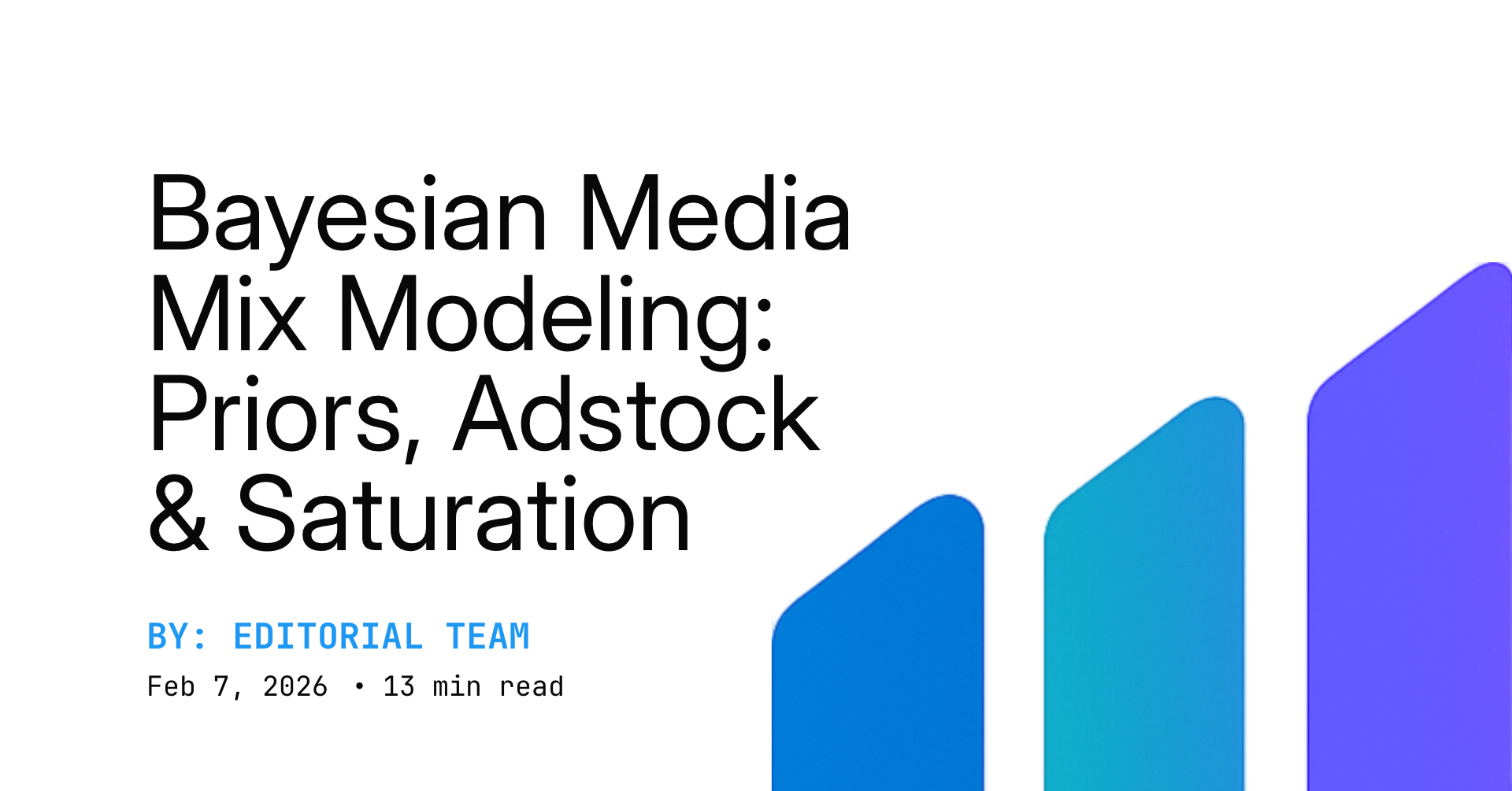
Before we dive into the solution, let’s look at the problem. Standard frequentist modeling (Ordinary Least Squares or OLS) relies entirely on the data you feed it.

If your data says spending went up and sales went down, the model assumes marketing hurts sales. It doesn't care that you had a stockout that week. It doesn't care that a competitor launched a massive promo.

It treats every variable as a blank slate.

This leads to volatile results. One month, Facebook looks like a goldmine. The next, it looks like a money pit. This instability makes it impossible to plan a budget with confidence. According to Harvard Business Review, relying solely on short-term data without context often leads to misallocation of resources.

You need a framework that handles uncertainty better. You need a system that incorporates what you already know about your business.

!Frequentist vs Bayesian modeling comparison chart showing confidence intervals.*

For a deeper dive into how this fits into your broader strategy, check out our media mix model marketing attribution guide.

What is Bayesian Media Mix Modeling?

Bayesian media mix modeling applies Bayes’ Theorem to marketing analytics.

In simple terms, it updates probabilities as more evidence becomes available.

A traditional model asks: "Based only on this dataset, what is the relationship between spend and revenue?"

A Bayesian model asks: "Given what we already know (Priors) and the new data we just observed (Likelihood), how should we update our belief about marketing performance (Posterior)?"

The Formula Simplified

• Prior: Your initial belief before seeing the data. (e.g., "TV usually has an ROI between 1.5 and 2.5").
• Likelihood: What the current data says.
• Posterior: The updated belief after combining the Prior and Likelihood.

You can explore the mathematical foundation of Bayes' Theorem here. This approach creates stable, realistic models. It prevents the model from producing impossible results, like negative coefficients for major ad platforms.

The Power of Priors

Priors are the superpower of bayesian media mix modeling. They allow you to inject human intelligence and external test results into the math.

Imagine you run a lift study on YouTube. The study proves a 10% incremental lift.

In a traditional model, you can't easily force the model to respect that 10% finding. If the daily data is noisy, the model might say YouTube did nothing.

In a Bayesian framework, you set a "Prior" for YouTube. You tell the model: "We are 90% sure the effect is positive, centered around a 10% lift."

The model then looks at the data. Unless the data overwhelmingly contradicts your belief (e.g., sales dropped to zero while spend tripled), the model will respect that lift study.

Types of Priors

• Uninformative Priors: You tell the model nothing. You let the data speak for itself. This mimics frequentist modeling.
• Informative Priors: You use previous MMM results, lift studies, or industry benchmarks to guide the model.

Using informative priors is essential when launching new channels where data is scarce. It stabilizes the model until enough history accumulates.

If you are struggling to compare different modeling approaches, read our MTA vs MMM comparison.

Adstock: Measuring the Memory of Marketing

Ads don't vanish from a consumer's mind the second they scroll past. They linger.

If you see a TV spot today, you might buy the product next week. If you stop spending today, sales won't drop to zero tomorrow. They decay over time.

This is called the Adstock effect.

Bayesian media mix modeling treats adstock as a parameter to be estimated. It calculates the "decay rate"—the percentage of the ad's effect that carries over to the next day. Academic research often utilizes distributed lag models to quantify this delayed impact mathematically.

Common Adstock Transformations

• Geometric Decay: The simplest form. The effect drops by a fixed percentage each day (e.g., 50% today, 25% tomorrow, 12.5% the next day).
• Weibull Delay: More complex but realistic. It allows for a delayed peak. Sometimes an ad needs to be seen a few times before it "hits." The effect builds up and then decays.

[IMAGE: Line graph illustrating Geometric Decay vs. Weibull Decay. Geometric starts high and drops. Weibull curves up slightly before dropping.]

Alt text: Visualizing Adstock: Geometric vs Weibull Decay rates.

!Visualizing Adstock: Geometric vs Weibull Decay rates.*

Saturation Curves: The Law of Diminishing Returns

You cannot spend your way to infinity.

The first $1,000 you spend on Facebook Ads usually targets your best audience. It yields high returns. The next $10,000 targets a slightly broader, less interested audience. Returns drop.

Eventually, you hit a wall where spending more yields zero extra revenue. This is saturation.

Bayesian media mix modeling uses saturation curves (often the Hill function or Michaelis-Menten function) to map this reality. These functions are standard in biology and economics to model diminishing returns.

Why The Shape Matters

• Linear (Bad): Assumes every dollar earns the same back. Leads to reckless overspending.
• Concave (Realistic): Shows returns flattening out.

S-Curve (Complex): Suggests you need a minimum spend to see any* result, then efficiency spikes, then it flattens.

The Bayesian approach estimates the shape of this curve for every channel. It tells you exactly where you sit on the curve. Are you in the efficient zone? Or are you burning cash in the saturated zone?

Understanding these curves is vital for media budget optimization.

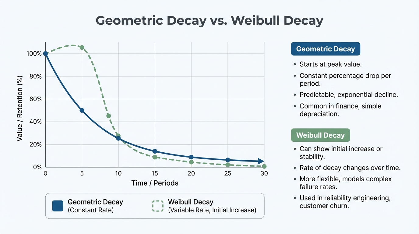
The Engine: MCMC Sampling

How does the model actually find the answer? It uses a technique called Markov Chain Monte Carlo (MCMC).

Think of MCMC as a robot exploring a mountain range in the dark.

• The robot takes a step (guesses a set of parameters).
• It checks if this spot fits the data better than the last spot.
• If yes, it stays. If no, it might stay anyway (to explore) or move back.
• It repeats this thousands of times.

Eventually, the robot maps out the entire "shape" of the solution. It doesn't just give you one answer. It gives you a distribution of likely answers. You can read more about the mechanics of MCMC sampling here.

This is why Bayesian models are computationally heavy but incredibly robust. They show you the probability of an outcome, not just a single guess.

This level of analysis is crucial when performing a detailed marketing ROI analysis.

[IMAGE: Diagram of MCMC sampling showing a chain of iterations converging on a probability distribution.]

Alt text: MCMC sampling process converging on a solution.

Caption: MCMC sampling allows the model to explore thousands of possibilities to find the most accurate fit.

!MCMC sampling process converging on a solution.*

Why should you switch? Here is the breakdown.

| Feature | Frequentist (OLS) | Bayesian |

| :--- | :--- | :--- |

| Input | Data only | Data + Priors (Business Context) |

| Stability | Volatile with noisy data | Stable, robust to noise |

| Output | Single point estimate | Probability distribution |

| Granularity | Struggles with many variables | Handles complex, high-dimension data |

| Updates | Re-run from scratch | Updates with new data |

For a detailed breakdown of different modeling methodologies, read our guide on which MMM is best.

Implementing Bayesian MMM

You have two main paths to deployment: Open Source or SaaS.

Open Source Options

Big tech has realized the value of bayesian media mix modeling.

• Google Meridian: Google’s next-gen model. It offers sophisticated Bayesian priors and geospatial modeling capabilities. You can view their official documentation here. Read our Google Meridian MMM guide for a simplified breakdown.
• Meta Robyn: An automated code library from Meta that uses Facebook’s Prophet for seasonality and Ridge regression within a Bayesian framework. Their GitHub repository is a great resource for data scientists. Check out our Meta Robyn guide for implementation tips.

These tools are powerful but require data science teams to operate. You need to clean the data, tune the hyperparameters, and interpret the MCMC chains yourself.

SaaS Solutions (BlueAlpha)

If you don't have a team of data scientists, platforms like BlueAlpha automate the heavy lifting.

BlueAlpha ingests your data, automatically selects the best priors based on your industry vertical, and runs the MCMC sampling in the cloud. It turns complex saturation curves into simple "Spend More / Spend Less" recommendations.

For a practical walkthrough, see how to deploy a media mix model.

Overcoming Data Challenges

A model is only as good as the data you feed it. Bayesian methods help smooth over gaps, but they aren't magic.

1. Granularity

You need daily or weekly data. Monthly data points are too few for the model to learn adstock effects accurately.

2. Collinearity

When you scale Facebook and Google spend up at the exact same time, the model struggles to tell which one caused the sales.

• Solution: Randomize your spend. Push one channel while holding the other steady.
• Bayesian Fix: Use priors from lift tests to separate the signals.

3. Seasonality

Sales spike in Q4 naturally. If you don't account for this, the model will think your Q4 ads are geniuses.

• Solution: Include seasonality variables (holidays, economy, weather).

For specific advice on B2B complexity, look at our account-based marketing attribution guide.

Interpreting the Output: Decomposition

Once the model runs, you get a Sales Decomposition.

This breaks down your total revenue into "Base" and "Incremental."

• Base: Sales you would get with zero marketing (brand equity, organic search, returning customers).
• Incremental: Sales driven specifically by marketing activities.

Bayesian models are excellent at separating Base from Incremental because they can use priors to constrain the "Base" to realistic levels. A frequentist model might erroneously claim your Base sales are negative, which is impossible.

[IMAGE: Stacked bar chart showing sales decomposition. Base sales at the bottom, layered with different marketing channels on top.]

Alt text: Marketing Mix Model Sales Decomposition Chart.

Caption: Decomposition shows exactly how much revenue each channel and baseline factors contribute.

!Marketing Mix Model Sales Decomposition Chart.*

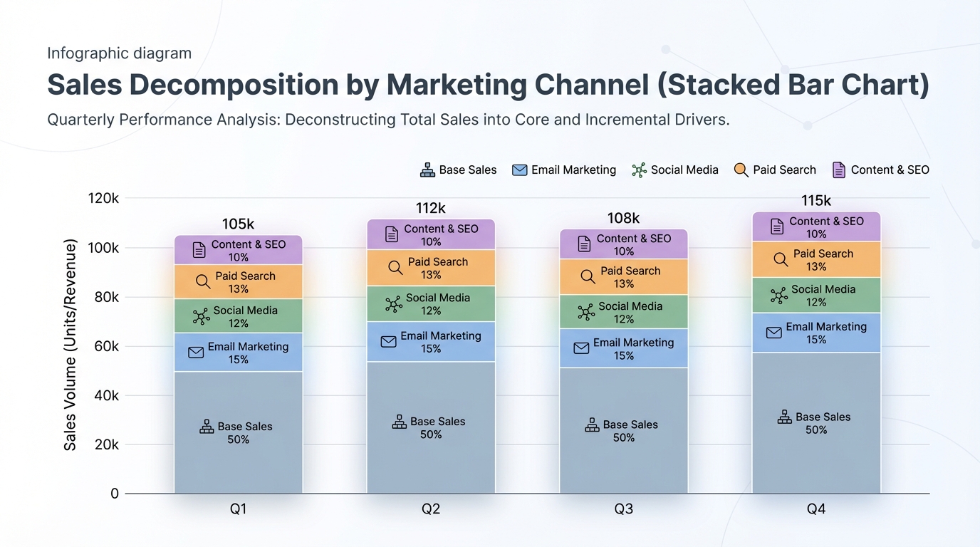
Measuring Hard-to-Track Channels

The biggest win for bayesian media mix modeling is tracking offline and upper-funnel activity.

Out of Home (OOH)

Billboards don't get clicks. But they do drive search volume. By feeding OOH spend data into the model and setting a prior based on location foot traffic, you can measure the lift.

Learn more:* Out of home advertising tracking guide.

Influencers

Influencer marketing is notoriously spiky. One post goes viral; the next flops. Bayesian models smooth these spikes using adstock to show the true cumulative value.

Learn more:* Influencer marketing performance measurement guide.

Comparison: BlueAlpha vs. The Market

When choosing a tool to implement Bayesian MMM, you have options. It helps to compare capabilities directly.

BlueAlpha focuses on automating the Bayesian workflow for speed and accuracy without the technical overhead.

• Vs. Funnel.io: Funnel is great for data aggregation, but it doesn't do the heavy modeling. See Funnel.io vs BlueAlpha.
• Vs. Triple Whale: Triple Whale is excellent for Shopify attribution (pixel-based), but MMM provides a broader view of offline and non-clickable impact. See Triple Whale vs BlueAlpha.
• Vs. Northbeam: Northbeam uses machine learning for attribution, but a dedicated Bayesian MMM offers more transparency into the "why" behind the numbers. See Northbeam vs BlueAlpha.
• Vs. Recast: Recast is a strong competitor in the Bayesian space. We break down the differences in our Recast vs BlueAlpha comparison.

Other platforms like Measured and Lifesight also offer measurement solutions, but often rely on different methodologies or incrementality testing focus rather than pure continuous MMM.

Best Practices for Bayesian Modeling

To get the most out of your model, follow these rules:

• Update Regularly: Marketing changes fast. Re-run your model weekly or monthly.
• Validate with Experiments: Run geo-lift tests. Use the results to update your Priors. This creates a feedback loop that makes the model smarter over time.
• Don't Overfit: A model that fits historical data 100% perfectly is usually wrong about the future. Bayesian methods help prevent this, but be wary of "perfect" R-squared values.
• Context is King: Always interpret results with business context. If the model says "stop bidding on brand keywords," check if competitors are bidding on your name first.

For companies looking at alternatives to their current stack, check our guides on Measured alternatives or Triple Whale alternatives.

Frequently Asked Questions (FAQ)

How much data do I need for Bayesian MMM?

Ideally, you need at least two years of historical data (weekly granularity) to capture seasonality. However, Bayesian models with strong priors can produce decent insights with as little as 6-12 months of data, unlike frequentist models which would fail.

Can Bayesian MMM replace Multi-Touch Attribution (MTA)?

They do different things. MTA tracks user paths (micro-view). MMM measures aggregate impact (macro-view). They work best together. MMM tells you how much to spend; MTA helps you optimize tactical creative and placement.

How do I determine the right Priors?

Start with "uninformative" priors if you know nothing. As you run lift studies (e.g., Facebook Lift, Geo-holdouts), use those results to tighten your priors. You can also use industry benchmarks provided by platforms like BlueAlpha.

Is Bayesian MMM expensive?

It used to be. Custom consulting projects cost $50k+. Now, automated SaaS solutions and open-source libraries have brought the cost down significantly, making it accessible to mid-market brands.

Why is Bayesian MMM becoming more popular now?

The decline of third-party cookies and privacy regulations have made tracking individual users difficult. The Google Privacy Sandbox initiative highlights this shift away from user-level tracking. Bayesian MMM does not rely on cookies, making it a future-proof solution.

Conclusion

Bayesian media mix modeling is the bridge between data science and marketing intuition.

It respects the complexity of consumer behavior. It accounts for the lingering effect of ads (Adstock) and the reality of budget limits (Saturation). Most importantly, it allows you to teach the model what you already know (Priors).

In a privacy-first world where cookies are dying and tracking is breaking, Bayesian MMM is not just a "nice to have." It is the future of measurement.

Stop guessing with your budget. Start modeling with probability.

Ready to see how Bayesian math can save your budget? Explore how BlueAlpha compares to other tools or dive deeper into our ABM ROI measurement guide.