Marketing data is messy. Cookies are crumbling. The old way of tracking every click to a conversion is dead.

You need a new source of truth.

Enter Media Mix Modeling (MMM). Specifically, Bayesian MMM using Python.

If you are a data scientist or a technical marketer, you’ve likely heard of PyMC Marketing. It’s the open-source library that brings the power of Bayesian statistics to marketing analytics. This pymc marketing tutorial cuts through the academic jargon. We will build a working model, interpret the results, and turn data into budget decisions.

Most guides get stuck in theory. We are going to focus on implementation.

Why Bayesian Media Mix Modeling Wins

Most legacy attribution tools look backward. They count clicks. But clicks don't equal influence.

Bayesian MMM is different. It measures incremental lift. It tells you what would have happened if you didn't spend that money.

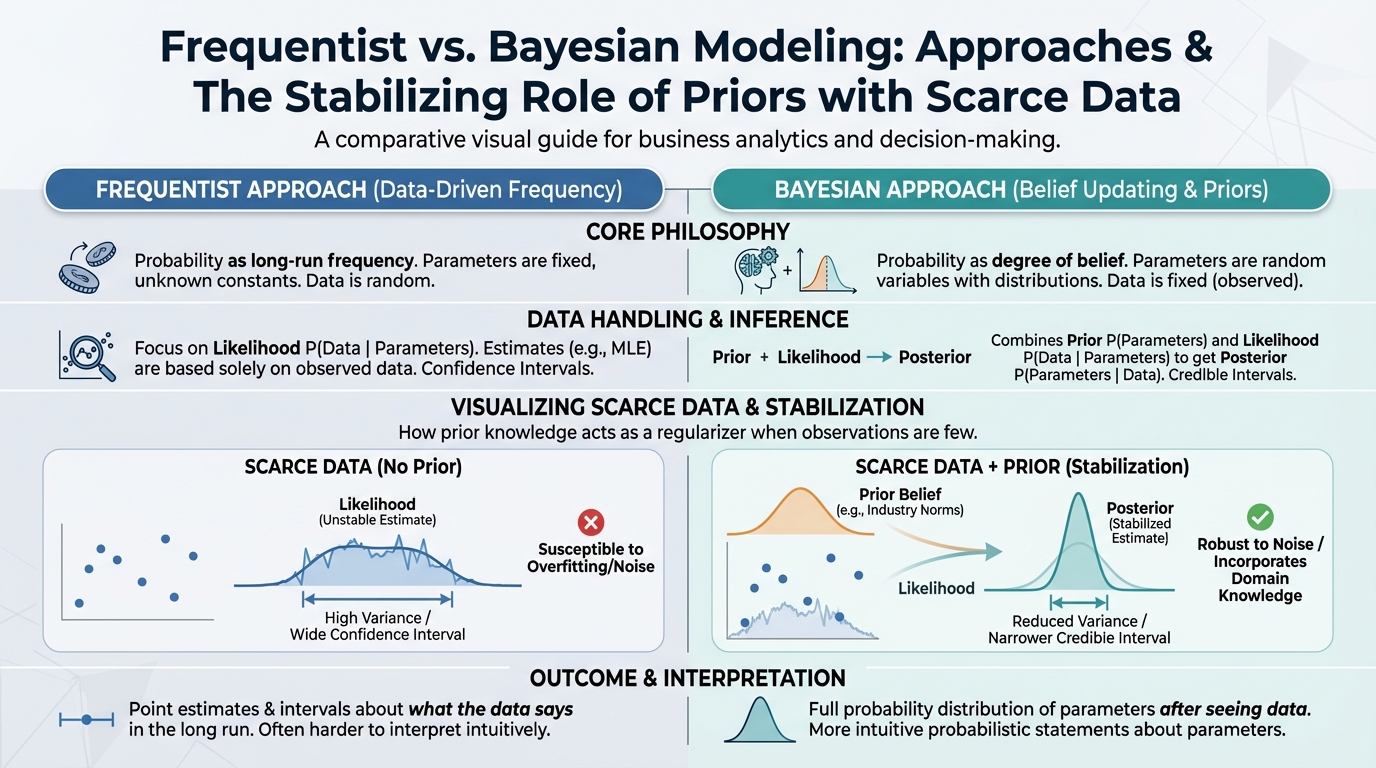
The Bayesian Difference

In frequentist statistics (the standard kind), you let the data speak entirely for itself. That sounds great until you have a small dataset or noisy signals. If you only have two years of weekly data, a standard regression model might tell you that spending $0 on Facebook is optimal because of one bad month.

Bayesian models allow you to use "priors." You can tell the model, "I know Facebook ads generally have a positive effect." The model then updates this belief based on your actual data.

This approach aligns perfectly with modern marketing effectiveness measurement. You aren't just fitting a line to a chart; you are modeling reality. Leading firms like McKinsey emphasize that integrating business expertise into models is crucial for accuracy.

PyMC Marketing vs. The Field

Google has Meridian. Meta has Robyn. Why use PyMC?

PyMC Marketing is built on top of PyMC, the standard for Bayesian modeling in Python. It offers granular control. You aren't stuck with a black box. You can customize adstock functions, saturation curves, and seasonality to fit your specific business logic.

While tools like Google Meridian offer robust features, PyMC Marketing provides a developer-first experience that integrates seamlessly into existing Python data stacks.

!Diagram contrasting frequentist regression lines with Bayesian probability distributions for marketing attribution.*

Prerequisites for Python for Marketing Analytics

Before we write code, ensure your environment is ready. You need Python installed (preferably 3.10+).

You will need the following libraries:

• pymc-marketing
• pandas
• numpy
• matplotlib or seaborn

Install them via pip:

pip install pymc-marketing pandas matplotlib

This pymc marketing tutorial assumes you understand basic Python syntax and data manipulation. If you are new to the data science ecosystem, familiarizing yourself with Pandas is a must.

Step 1: Data Preparation

Garbage in, garbage out. This is the golden rule of data science.

Your data must be aggregated. MMM works on a time-series basis (usually weekly). You cannot feed it user-level data.

Structure Your DataFrame

You need a CSV or DataFrame with columns for:

• Date: Weekly granularity is standard.
• Target: Revenue or Conversions.
• Media Variables: Spend or Impressions for each channel (FB, Google, TV, TikTok).
• Control Variables: Organic traffic, price changes, holidays, competitor activity.

If you are transitioning from Multi-Touch Attribution (MTA), this aggregation step is the biggest shift. You can read more about the differences in our MTA vs MMM comparison.

import pandas as pd
Load your data
df = pd.read_csv('marketing_data.csv')
Ensure your date column is datetime objects
df['date'] = pd.to_datetime(df['date'])
Set date as index (often required for plotting/splitting)
df.set_index('date', inplace=True)

Step 2: Understanding Adstock and Saturation

MMM relies on two core concepts: Adstock and Saturation.

Adstock (The Lag Effect)

If you see a TV ad today, you might buy a car next week. The effect of the ad "decays" over time.

• Geometric Adstock: A simple fixed decay rate.

Weibull Adstock: Allows the peak effect to happen after* the initial exposure (common for brand campaigns).

Saturation (Diminishing Returns)

Spending \$100k is great. Spending \$100M in a week is wasteful. Eventually, everyone has seen your ad. The next dollar yields less revenue than the first. We model this using a curve (often a Michaelis-Menten or Hill function)).

Properly modeling these curves is essential for accurate marketing ROI analysis. If you assume linear growth, you will overspend.

[IMAGE: Diagram illustrating Adstock decay and Saturation curves. Left side: Bar chart showing ad effect lingering over weeks. Right side: S-curve showing diminishing returns.]

Alt text: Visual explanation of Geometric Adstock decay and Hill function saturation curves in media mix modeling.

!Visual explanation of Geometric Adstock decay and Hill function saturation curves in media mix modeling.*

Now, let’s use PyMC Marketing. The library provides a high-level API that abstracts away the complex math while keeping the Bayesian engine running.

We will use the MMM class.

from pymc_marketing.mmm import MMM
Define column names
date_col = "date"
channel_cols = ["fb_spend", "google_spend", "tiktok_spend"]
control_cols = ["holidays", "competitor_price"]
target_col = "revenue"
Initialize the model
mmm = MMM(
adstock="geometric",  # or 'weibull'
saturation="logistic", # or 'hill'
date_column=date_col,
channel_columns=channel_cols,
control_columns=control_cols,
adstock_max_lag=8, # How many weeks does the ad effect last?
yearly_seasonality=2, # Fourier order for seasonality
)

Setting Priors

This is where the "Bayesian" part happens. You don't have to accept the defaults.

If you know that Google Search is your strongest channel, you can set a higher prior for its contribution. If you are comparing Meta Robyn vs. open source MMM, you'll find that PyMC's flexibility in defining custom priors is a major advantage for teams with deep institutional knowledge.

Step 4: Training the Model

Training involves "sampling." The model tries thousands of different parameter combinations to find the distribution that best explains your data.

# Fit the model to the data
mmm.fit(df, target_column=target_col)

This process uses MCMC (Markov Chain Monte Carlo). It might take a few minutes depending on your data size. The underlying engine, maintained by PyMC Labs, ensures that the sampling is robust and mathematically sound.

Diagnostics

Once trained, you must check if the model converged. In Bayesian stats, we look for "divergences" or check the "R-hat" statistic.

• R-hat < 1.05: Good. The chains mixed well.
• R-hat > 1.1: Bad. The model is confused. You may need more data or better priors.

For a deeper dive on validating these models, check our guide on how to deploy media mix models.

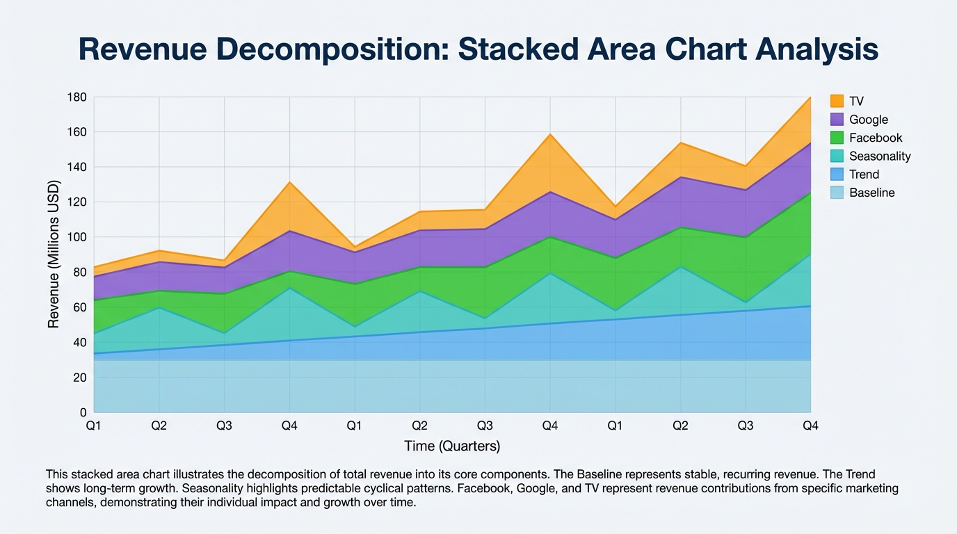
Step 5: Visualizing Contributions

The model is trained. Now, what drove sales?

PyMC Marketing has built-in plotting tools to visualize the decomposition of your target variable.

mmm.plot_components_contributions();

This generates a chart showing how much revenue was driven by:

• Trend: The baseline growth of your company.
• Seasonality: Yearly cycles.
• Media Channels: The incremental lift from ads.
• Controls: External factors.

This visual is critical for stakeholders. It moves the conversation from "I think TV worked" to "The model shows TV contributed $500k in incremental revenue."

[IMAGE: Stacked area chart showing revenue decomposition. Layers for Baseline, Trend, Seasonality, Facebook, Google, and TV.]

Alt text: Marketing mix model decomposition chart showing baseline sales versus media contributions.

Caption: Decomposing revenue helps identify the true incremental lift of each marketing channel.

!Marketing mix model decomposition chart showing baseline sales versus media contributions.*

This is the "So What?" of the pymc marketing tutorial.

You have a model. Now you want to know: How should I spend my budget next quarter?

The goal is to maximize revenue for a given budget constraint. Because we modeled saturation curves, the model knows that moving money from a saturated channel (Facebook) to an unsaturated one (TikTok) will increase total returns.

# Optimize budget for next quarter
optimal_budget = mmm.optimize_budget(
total_budget=1000000,
num_periods=12
)
print(optimal_budget)

This output gives you the mathematical ideal. However, you must apply human judgment. You cannot simply shut off a channel because the model says so—you might lose brand presence that the model hasn't captured yet.

This aligns with broader strategies for media budget optimization, where algorithmic suggestions meet strategic constraints.

Advanced Considerations

Handling Funnel Stages

Standard MMM flattens everything to "Revenue." But B2B companies often have long sales cycles. You might want to model "Leads" or "Opportunities" instead of cash.

If you are in B2B, you should structure your data to reflect different stages. See our funnel stage budget allocation guide for details on mapping spend to specific funnel outcomes.

Out-of-Sample Testing

Never trust a model that has only seen the training data. Always hold back the last 4-8 weeks of data. Predict those weeks using the model. If the prediction matches reality, your model is robust.

According to research from Harvard Business Review, companies that rigorously validate their analytics models and integrate them into strategy see significantly higher marketing efficiency. Validation isn't optional; it's the difference between a guess and a prediction.

Incorporating Experiments

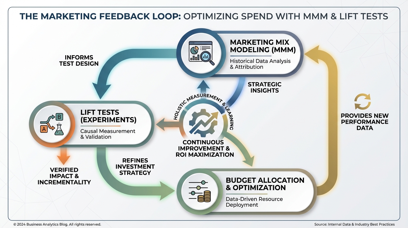
The gold standard is calibrating your MMM with lift tests. Run a geo-lift test (turn off ads in Ohio). Feed that result back into the model as a prior.

This concept creates a feedback loop. The MMM guides the strategy, experiments validate the MMM, and the model gets smarter. This is particularly useful when dealing with hard-to-track channels, as discussed in our out-of-home advertising tracking guide.

[IMAGE: Process diagram showing the feedback loop between MMM, Lift Tests, and Budget Allocation.]

Alt text: Diagram showing how lift tests calibrate MMM priors for better budget allocation.

Caption: Calibrating your PyMC model with real-world lift tests drastically improves accuracy.

!Diagram showing how lift tests calibrate MMM priors for better budget allocation.*

Building a custom solution with PyMC Marketing is powerful, but it is not free. The cost is engineering time.

The Maintenance Burden

Data pipelines break. APIs change. Internal stakeholders ask for "what-if" scenarios that require recoding the model. You need a dedicated data scientist to maintain this. If that person leaves, your attribution model leaves with them.

Organizations like Gartner frequently highlight the "hidden costs" of internal build projects, specifically regarding technical debt and maintenance.

Processing Speed

MCMC sampling is computationally expensive. As your data grows, training times increase. You may need to optimize your PyTensor code or move to GPU acceleration.

When to Buy Instead of Build

If you are a massive enterprise with a data science team of 20, building with PyMC is a great move.

For mid-market companies or lean growth teams, the overhead often outweighs the benefits. This is where managed platforms come in. Solutions like BlueAlpha wrap the power of Bayesian modeling in a user-friendly interface with faster implementation times and dedicated support. You get the sophisticated math of PyMC without the maintenance burden or technical debt.

We’ve compared various managed options to help you decide. For example, check out Recast vs. BlueAlpha or Measured.com vs. BlueAlpha to see how managed services stack up against building it yourself.

Conclusion

PyMC Marketing represents a massive leap forward for open-source analytics. It democratizes access to sophisticated Bayesian statistics.

By following this pymc marketing tutorial, you’ve learned how to:

• Structure your data for MMM.
• Define Adstock and Saturation.
• Train a Bayesian model using PyMC.
• Optimize your marketing budget based on data.

The era of guessing is over. Whether you build your own model in Python or use a platform to accelerate the process, the math is clear: Bayesian MMM is the future of marketing measurement.

Ready to skip the setup and get results faster? See how BlueAlpha can deliver the same insights without the engineering overhead.

---

Frequently Asked Questions (FAQ)

What is the difference between PyMC Marketing and LightweightMMM?

LightweightMMM was a library developed by Google based on Numpyro. However, Google has largely shifted focus to Meridian. PyMC Marketing is maintained by PyMC Labs and the open-source community, offering tighter integration with the PyMC ecosystem and more flexibility in defining custom priors.

How much data do I need for PyMC Marketing?

Ideally, you need at least two years of weekly data (104 data points) to capture seasonality effectively. However, because it is Bayesian, you can get usable results with less data if you use strong, informed priors.

Can PyMC Marketing measure brand equity?

Yes, by using the "intercept" or baseline of the model. You can also incorporate brand tracking metrics (like share of search or brand sentiment) as control variables to see how brand health impacts baseline sales.

Is PyMC Marketing free?

Yes, the library is open-source and free to use under the Apache 2.0 license. However, you pay for the compute resources to run it and the engineering time to maintain it.

How does this compare to multi-touch attribution (MTA)?

MTA tracks user paths, which is becoming impossible due to privacy changes (iOS 14+, cookie deprecation). MMM is privacy-safe because it uses aggregated data. For a detailed breakdown, read our marketing attribution guide.